pak::pak("tdscience/tartu26")Analysing spatio-temporal origin-destination data
1 Install the required packages
See the prerequisites page on ways to install and setup an environment with the R packages needed to run the code in this workbook.
You are welcome to implement the work presented here in another language if you have the motivation and skills to do so. See the python-based workbook for an example of origin-destination data generation and processing in Python, for example.
library(spanishoddata)
library(flowmapblue)
library(mapgl)
library(tidyverse)
library(sf)
library(tmap)
tmap_mode("view")
2 Download and prepare the data
The example builds on the code in the Prerequisites section (see demo.qmd for a minimal example).
2.1 Northern Spain case study: Pamplona to Donostia corridor
In this workbook you will explore mobility patterns in Northern Spain, covering the Basque Country and Navarre regions. This area includes the cities of Pamplona (Iruña) and Donostia (San Sebastián). It forms a roughly rectangular study area from the border between Spain and France in the East to the edge of the Bilbao to the West.
Rather than filtering by a text pattern (as we did in the demo for Seville), we define the study area geographically with a bounding box and select all districts that intersect it. This approach allows you to run the code below for other regions; if you do choose a different case study area you could choose an alternative to the border between Spain and France as the basis for analysing flows between a linear feature, e.g. a major road, railway or river reducing connectivity between settlements.
The province codes in the zone
id field can also be used: Navarre = 31, Gipuzkoa = 20, Bizkaia = 48, and Álava = 01. The OD data we will be using from the Spanish Ministry of Transport was released in different versions, with the 2nd being more up-to-date, explaining the argument ver = 2 in the code chunks below.
spod_set_data_dir('data')
# Get zones
zones <- spod_get_zones(zones = "distr", ver = 2)
valid_dates <- spod_get_valid_dates(ver = 2)
recent_dates = tail(valid_dates, 3)

# Define a geographic bounding box for the Northern Spain study area
# Covers from the coast to south of Pamplona, and from the French border
# westward to include the Pamplona--Donostia corridor
bbox_north <- st_bbox(c(xmin = -3.1, ymin = 42.8, xmax = -1.0, ymax = 43.4), crs = st_crs(4326))
bbox_sf <- st_as_sfc(bbox_north)

# Select zones that intersect the bounding box
sf::sf_use_s2(FALSE)
zones_wgs84 <- st_transform(zones, 4326)
zones_north <- zones_wgs84 |>
  st_filter(bbox_sf, .predicate = st_intersects)

# Visualise the selected zones:
# plot(st_geometry(zones_north)) # basic plot
qtm(zones_north) + qtm(bbox_sf)

# Prepare location data (centroids) for the flow map
locations_north <- zones_north |>
  st_centroid() |>
  st_coordinates() |>
  as.data.frame() |>
  mutate(id = zones_north$id) |>
  rename(lon = X, lat = Y)
The following code chunk download the OD data for the recent dates and filters, to the zones in our study area, and aggregates by hour to create a spatio-temporal dataset suitable for animation. For workshop use, we have precomputed this dataset and saved it as an RDS file, so you can skip the this chunk.
Data download and preparation code (unfold this code chunk if you want to download and process datasets for another case study with different spatial and temporal bounds)
system.time({
flows <- spod_get(
  type = "origin-destination",
  zones = "districts",
  dates = recent_dates
)

od_data_time <- flows |>
  mutate(time = as.POSIXct(paste0(date, "T", hour, ":00:00"))) |>
  group_by(origin = id_origin, dest = id_destination, time) |>
  summarise(count = sum(n_trips, na.rm = TRUE), .groups = "drop") |>
  collect()

flows_north_time <- od_data_time |>
  filter(origin %in% zones_north$id & dest %in% zones_north$id)
})
# Save as arrow:
arrow::write_parquet(flows_north_time, "flows_north_time.parquet")
arrow::write_parquet(locations_north, "locations_north.parquet")
Downloaded the datasets we have prepared by navigating to github.com/tdscience/tartu26/releases in your browser, or use the code below to download the code programatically.
With the gh command line interface (CLI)
If you have the gh CLI installed (you probably don’t if you don’t know what this is), run this command from your system shell, e.g. PowerShell or a terminal:
gh release download v1 --repo tdscience/tartu26With R
message("Precomputed Northern Spain data not found.")
# Download from GitHub release assets:
# system("gh release download v1 --pattern 'flows_north_time.rds'")
release_url <- "https://github.com/tdscience/tartu26/releases/download/v1/"
for(f in c("flows_north_time.rds", "locations_north.rds")) {
  if (!file.exists(f)) download.file(paste0(release_url, f), f, mode = "wb")
}
3 Generate the interactive flow map
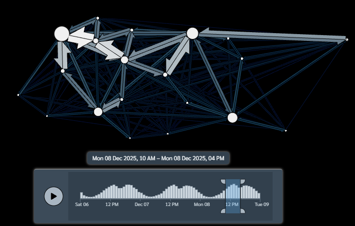
3.1 Northern Spain flow map
locations_north <- readRDS("locations_north.rds")
flows_north_time <- readRDS("flows_north_time.rds")
flowmap_north_interactive <- flowmapblue(
  locations = locations_north,
  flows = flows_north_time,
  mapboxAccessToken = Sys.getenv("MAPBOX_TOKEN"),
  darkMode = TRUE,
  animation = FALSE,
  clustering = TRUE
)

# Display the map
flowmap_north_interactive
The resulting interactive map is shown in Figure 1.
Getting a Mapbox token
4 Setting up Mapbox Access Token
Get a free token from https://account.mapbox.com/access-tokens/
Or, longer term solution: usethis::edit_r_environ() Restart R after setting the token for it to take effect
Sys.setenv(MAPBOX_TOKEN="YOUR_MAPBOX_ACCESS_TOKEN")
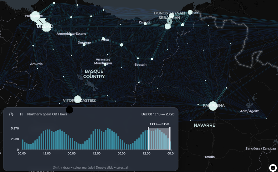
Bonus exercise: Northern Spain flow map using mapgl
Alternatively, we can use the mapgl package to visualize the Northern Spain flows using high-performance WebGL rendering. This operates entirely within the browser without requiring a Mapbox account, and adds an interactive timeline scrubber to explore the spatio-temporal trends.
This approach is a bonus exercise and designed to showcase the capabilities of mapgl for spatio-temporal flow maps, but it requires a version of the package from the e-kotov R-universe repository that includes the add_time_control() function.
# Note: this code block requires a version of the mapgl package from the e-kotov R-universe repository, which includes the add_time_control() function for spatio-temporal flow maps.
install.packages('mapgl', repos = c('https://e-kotov.r-universe.dev', 'https://cloud.r-project.org'))
library(mapgl)

# Create the MapLibre map centered on the Northern Spain corridor
north_mapgl <- maplibre(
  style = carto_style("dark-matter"),
  center = c(-1.75, 43.05),
  zoom = 8.5,
  projection = "mercator"
) |>
  add_flowmap(
    id = "north-flows",
    locations = locations_north,
    flows = flows_north_time,
    flow_time_column = "time",
    flow_color_scheme = "Teal",
    flow_dark_mode = TRUE
  ) |>
  add_time_control(
    data = flows_north_time,
    time_column = "time",
    time_interval = "hour",
    title = "Northern Spain OD Flows"
  )

# Display the map
north_mapgl
You should see something like this (as shown in Figure 2):
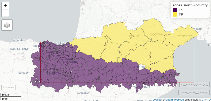
5 Cross-border analysis: Spain–France border effect
One of the most interesting research questions we can tackle with the Northern Spain study area is: to what extent does the national border between Spain and France act as a barrier to human mobility? The v2 spanishoddata data includes French zones (with IDs starting FR) alongside Spanish zones, making it possible to quantify the “border deterrence effect” – the reduction in travel attributable to the presence of an international boundary, after controlling for distance.
5.1 Approach
Our analysis proceeds in five steps:
- Identify French and Spanish zones in the study area using the zone ID prefix (
FR= France, all-numeric = Spain). - Classify each OD pair as cross-border (ES–FR), within-Spain (ES–ES), or within-France (FR–FR).
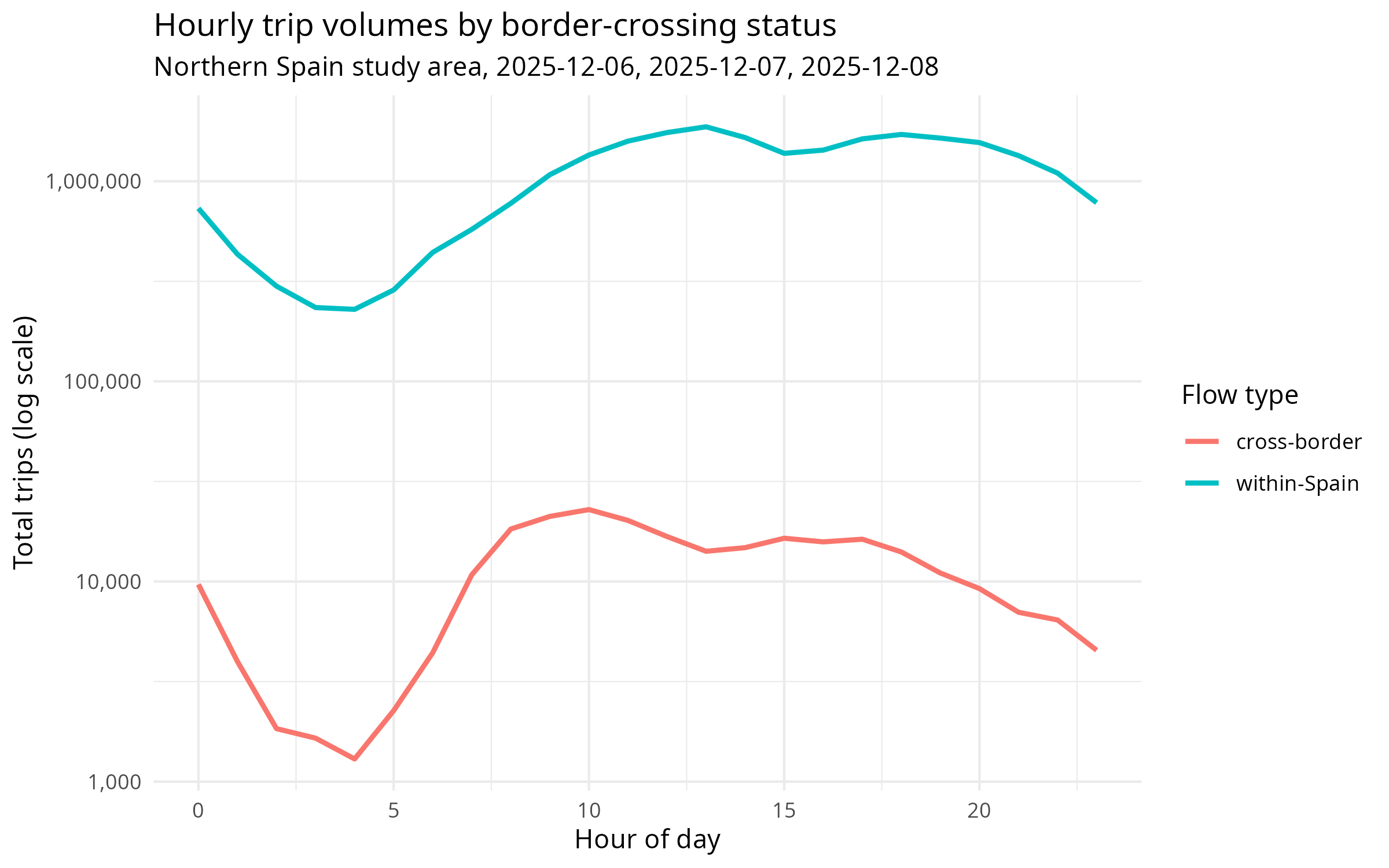
- Aggregate trip volumes by hour and border-crossing status to reveal temporal patterns.
- Estimate the border effect by comparing trip counts at comparable distances: for each distance band, what is the ratio of within-Spain trips to cross-border trips?
- Visualise the results as a distance-decay comparison plot.
We’ll use a larger area to cover a roughly equal area of Spain and France, as shown in Figure 3.
# ── 1. Load zones and classify by country ──────────────────────────────
sf::sf_use_s2(FALSE)
zones <- spod_get_zones(zones = "distr", ver = 2)

# Recreate larger area covering all the border between Spain and France, then select zones that intersect it:
bbox_north <- st_bbox(c(xmin = -3.1, ymin = 42.0, xmax = 4.0, ymax = 43.4), crs = st_crs(4326))
bbox_sf <- st_as_sfc(bbox_north)
zones_wgs84 <- st_transform(zones, 4326)
zones_north <- zones_wgs84 |>
  st_filter(bbox_sf, .predicate = st_intersects)

# Tag each zone by country
zones_north <- zones_north |>
  mutate(country = ifelse(grepl("^FR", id), "FR", "ES"))

cat("Zones in study area:", nrow(zones_north), "\n")
cat("  Spanish:", sum(zones_north$country == "ES"), "\n")
cat("  French: ", sum(zones_north$country == "FR"), "\n")
mapview::mapview(zones_north, zcol = "country", legend = TRUE) + mapview::mapview(st_geometry(bbox_sf), color = "red", alpha.regions = 0, lwd = 2)

# ── 2. Get OD data and classify each pair ───────────────────────────
valid_dates <- spod_get_valid_dates(2)
recent_dates <- tail(valid_dates, 3)

flows <- spod_get(
  type = "origin-destination",
  zones = "districts",
  dates = recent_dates
)

# Build a lookup table: zone ID → country
zone_country <- zones_north |>
  st_drop_geometry() |>
  select(id, country)

# Filter to study-area zones and tag each OD pair
od_north <- flows |>
  filter(
    id_origin %in% zones_north$id,
    id_destination %in% zones_north$id
  ) |>
  collect() |>
  left_join(zone_country, by = c("id_origin" = "id")) |>
  rename(country_origin = country) |>
  left_join(zone_country, by = c("id_destination" = "id")) |>
  rename(country_dest = country) |>
  mutate(
    border_crossing = case_when(
      country_origin != country_dest ~ "cross-border",
      country_origin == "ES"         ~ "within-Spain",
      country_origin == "FR"         ~ "within-France"
    )
  )

# ── 3. Temporal patterns by border status ──────────────────────────
hourly_by_border <- od_north |>
  group_by(hour, border_crossing) |>
  summarise(
    total_trips = sum(n_trips, na.rm = TRUE),
    .groups = "drop"
  ) |>
  collect()

# Plot: trip volumes by hour, faceted by border status
ggplot(hourly_by_border, aes(x = hour, y = total_trips, colour = border_crossing)) +
  geom_line(linewidth = 1) +
  scale_y_log10(labels = scales::comma) +
  labs(
    title = "Hourly trip volumes by border-crossing status",
    subtitle = paste("Northern Spain study area,",
                     paste(recent_dates, collapse = ", ")),
    x = "Hour of day",
    y = "Total trips (log scale)",
    colour = "Flow type"
  ) +
  theme_minimal()
ggsave("images/hourly_border_flows.png", width = 8, height = 5)
# ── 4. Distance-decay comparison ───────────────────────────────────
# Compare within-Spain vs cross-border flows at similar distances
dist_comparison <- od_north |>
  group_by(distance, border_crossing) |>
  summarise(
    total_trips = sum(n_trips, na.rm = TRUE),
    n_pairs     = n(),
    .groups     = "drop"
  ) |>
  collect()
The hourly trip volumes are compared in Figure 4.
5.2 Interpretation
- Temporal pattern: Cross-border flows typically show a flatter daily profile than within-Spain commuting flows, suggesting more leisure/tourism travel and less routine commuting across the border.
- Distance-decay: The
deterrence_ratiocolumn shows how many more within-Spain trips occur than cross-border trips at the same distance. A ratio of, say, 10× at the 10–20 km band means there are 10 times more trips between Spanish zones 15 km apart than between a Spanish and French zone 15 km apart. - Key question: At what distance does the border effect become negligible? If the ratio approaches 1 at longer distances, the border may primarily suppress short-distance local trips.
5.3 Further exploration
- Repeat the analysis for weekdays vs weekends to see if cross-border commuting is more common on certain days.
- Use the
activity_originfield to see whether cross-border trips are predominantly work, leisure, or study-related. - Expand the study area westward to include Bilbao and compare the border effect at Irun/Hendaye (major crossing) versus more remote Pyrenean crossings.
- Download a full month of data and examine how the border effect changes on public holidays and during school vacations.
6 Spatial analysis: Elevation profile and flow correlation
In this section, we analyze the spatial relationship between the physical geography of the region (elevation) and human mobility flows. We define a Southwest-to-Northeast transect line across our study corridor, segment it into 100 equal-length chunks, extract the average elevation for each chunk from a digital elevation model (DEM), and correlate this physical feature with the aggregate travel flows in the corresponding districts.
6.1 Download and load elevation data
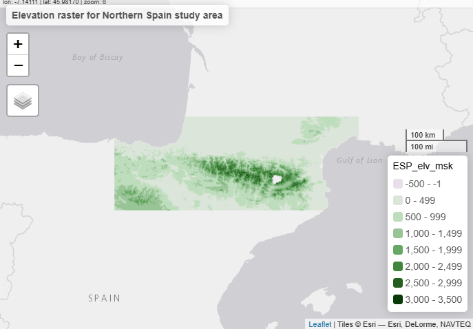
We use a low-resolution Digital Elevation Model (DEM) of Spain, cropped to the Northern Spain study area. The file is hosted as a GitHub Release asset for quick and reliable download.
if (!file.exists("spain_france_elevation.tif")) {
  release_url <- "https://github.com/tdscience/tartu26/releases/download/v1/spain_france_elevation.tif"
  download.file(release_url, "spain_france_elevation.tif", mode = "wb")
}

library(sf)
library(terra)
library(tidyverse)
library(spanishoddata)
library(tmap)

elev <- rast("spain_france_elevation.tif")
qtm(elev) + tm_layout(main.title = "Elevation raster for Northern Spain study area")
The loaded DEM is displayed in Figure 5.
6.1.1 Exercise
Read the code that download the data and add data for Andorra to avoid the gap in the DEM at the Spain–France border.
6.2 Segmentize the transect line
We define the transect line from \((-1.8, 43.3)\) to \((1.8, 42.3)\) in WGS84 coordinates to follow the French-Spanish border in a straight line with roughly half of it in each country. To partition it into equal-length spatial chunks, we project it to UTM Zone 30N (EPSG:25830) and sample points along it to construct 100 individual segments of equal length.
# Create the transect line in WGS84
line <- st_linestring(matrix(c(-1.8, 1.8, 43.3, 42.3), ncol = 2)) |>
  st_sfc(crs = 4326) |>
  st_sf(geometry = _)

# Project to UTM 30N for equal-length segmentation
line_proj <- st_transform(line, 25830)
pts <- st_line_sample(line_proj, n = 101) |> st_cast("POINT")

# Construct 100 individual line segments (chunks)
segments <- list()
for (i in 1:100) {
  segments[[i]] <- st_linestring(rbind(st_coordinates(pts[i]), st_coordinates(pts[i+1])))
}
segments_sf <- st_sfc(segments, crs = 25830) |> st_sf(segment_id = 1:100, geometry = _)

# Transform segments back to WGS84 for extraction and overlay
segments_wgs84 <- st_transform(segments_sf, 4326)
6.3 Extract elevation and associate with mobility flows
For each chunk, we calculate the average elevation from the DEM. We then identify which district/zone each chunk’s centroid falls into and join the total origin trip volume (flow) for that district.
# Extract average elevation for each segment
elev_vals <- terra::extract(elev, vect(segments_wgs84), fun = mean, na.rm = TRUE)
segments_wgs84$elevation <- elev_vals[, 2]

# Map segments to districts using their centroids
spod_set_data_dir('data')
zones <- spod_get_zones(zones = "distr", ver = 2)
bbox_north <- st_bbox(c(xmin = -3.1, ymin = 42.0, xmax = 4.0, ymax = 43.4), crs = 4326)
bbox_sf <- st_as_sfc(bbox_north)
zones_wgs84 <- st_transform(zones, 4326)
sf_use_s2(FALSE)
zones_north <- zones_wgs84 |> st_filter(bbox_sf, .predicate = st_intersects)

segments_centroid <- st_centroid(segments_wgs84)
segments_zone <- st_join(segments_centroid, zones_north)
segments_wgs84$zone_id <- segments_zone$id

# Calculate flow for each zone from the precomputed dataset
flows_north_time <- readRDS("flows_north_time.rds")
zone_flows <- flows_north_time |>
  group_by(origin) |>
  summarise(total_flow = sum(count, na.rm = TRUE), .groups = "drop")

# Join flow data and handle missing data
segments_final <- segments_wgs84 |>
  left_join(zone_flows, by = c("zone_id" = "origin")) |>
  replace_na(list(total_flow = 0, elevation = 0))

# Calculate Pearson correlation coefficient
cor_val <- cor(segments_final$elevation, segments_final$total_flow, use = "complete.obs")
cat(paste("Pearson Correlation between Elevation and Flow:", round(cor_val, 4), "\n"))
6.4 Visualization
We plot the elevation raster alongside the study zones and transect line (Map), the elevation profile along the line, and the relationship between elevation and flow.
# Define start and end point labels for the map
transect_points <- st_sfc(
  st_point(c(-1.8, 43.3)),
  st_point(c(1.8, 42.3)),
  crs = 4326
) |> st_sf(name = c("Start", "End"), geometry = _)

# A. Create the static Map using tmap
current_mode <- tmap_mode("plot")
map_plot <- tm_shape(elev) +
  tm_raster(col.scale = tm_scale_continuous(values = "terrain"),
            col.legend = tm_legend("Elevation (m)")) +
  tm_shape(zones_north) +
  tm_borders(col = "black", lwd = 0.5) +
  tm_shape(line) +
  tm_lines(col = "blue", linewidth = 3) +
  tm_shape(transect_points) +
  tm_symbols(size = 0.5, col = "red") +
  tm_text("name", ymod = 0.5)

print(map_plot)
tmap_mode(current_mode)

# B. Plot the elevation profile
# Calculate distance along the line from the start point (in km)
start_pt <- st_sfc(st_point(c(-1.8, 43.3)), crs = 4326) |> st_transform(25830)
segments_final_proj <- st_transform(segments_final, 25830)
segments_final$dist_km <- as.numeric(st_distance(st_centroid(segments_final_proj), start_pt)) / 1000

p_elev <- ggplot(segments_final, aes(x = dist_km, y = elevation)) +
  geom_line(color = "darkgreen", linewidth = 1) +
  geom_point(color = "darkgreen", size = 1.5) +
  labs(
    title = "Elevation Profile Along the Transect Line",
    x = "Distance from Start (km)",
    y = "Average Elevation (m a.s.l.)"
  ) +
  theme_minimal()
print(p_elev)

# C. Plot the elevation vs flow correlation
p_cor <- ggplot(segments_final, aes(x = elevation, y = total_flow)) +
  geom_point(color = "blue", alpha = 0.6, size = 2) +
  geom_smooth(method = "lm", color = "red", se = TRUE) +
  scale_y_continuous(labels = scales::comma) +
  labs(
    title = "Correlation: Elevation vs District Flow",
    subtitle = paste("Pearson Correlation:", round(cor_val, 4)),
    x = "Average Elevation (m a.s.l.)",
    y = "Total Zone Origin Flow"
  ) +
  theme_minimal()
print(p_cor)
7 Research questions
Below are suggested research questions you can explore with the spanishoddata package and the tools introduced in this workbook. They range from descriptive to analytical and are designed to be tractable within a short workshop or assignment.
Temporal commuting patterns – How do morning and evening peak flows differ between weekdays and weekends? Can you identify distinct commuter corridors within your chosen study area?
Cross-border mobility – The v2 data includes trips to and from France. What proportion of flows in the Northern Spain study area cross the international border, and how does this vary by time of day? (See the cross-border analysis section above for a worked example.)
Socio-demographic differences – Using the
income,age, andsexvariables available in v2, do flow patterns differ between demographic groups? For example, do higher-income groups travel further or at different times?Functional urban area definition – Compare the 10 km buffer approach used for Seville with the bounding-box approach used for Northern Spain. How sensitive are the resulting flow patterns to the choice of study area boundary?
Activity-purpose flows – The
activity_originandactivity_destinationfields classify trips by purpose (home, work, regular, irregular, study). What is the dominant flow purpose in your study area, and how does the spatial structure of work-related flows differ from leisure-related flows?Intra-zonal vs inter-zonal trips – Intra-zonal trips (where origin equals destination) often dominate OD datasets. What share of trips are intra-zonal in your study area, and how does excluding them change the visual pattern of the flow map?
Seasonal or special-event variation – If you download data for multiple time periods, can you detect changes in mobility associated with public holidays, festivals (e.g., San Fermín in Pamplona), or seasonal tourism patterns along the coast?
Comparative urban analysis – Replicate the analysis for both Seville and Northern Spain. Which city has higher average trip distances? Which shows more polycentric flow patterns (multiple distinct centres rather than a single dominant hub)?
8 Bonus Exercise: Contributing via Pull Request
A key skill in collaborative data science is contributing improvements, fixes, or new examples to open-source project repositories using Git and GitHub.
In this bonus exercise, you will create a Pull Request (PR) to this repository:
Find something to improve: This could be correcting a typo in the documentation, adding a comment to clarify a complex code block, or contributing a new research question/exercise.
Create a branch: In your local terminal or Codespace, create a new branch:
git checkout -b my-improvement-branchCommit your changes: Stage and commit your changes:
git add .
git commit -m "docs: Fix typo in workbook"
Push and Open a Pull Request: Push your branch to GitHub and open a Pull Request.
For a detailed step-by-step walkthrough, check out the following official guides:
- GitHub Flow Guide: An introduction to branching, committing, and opening PRs.
- Collaborating with pull requests: The official GitHub guide on how to propose changes.
- Forking a repository: If you do not have direct push access, learn how to fork, make changes, and open a PR back to the main repository.
9 Further resources
This workbook builds on the tutorial “Analysing massive open human mobility data in R using spanishoddata, duckdb and flowmaps” (Kotov 2025), and the spatio-temporal data session in the Data Science for Transport Planning course. For a detailed description of the dataset and its potential applications, see the original paper introducing the spanishoddata package (Kotov et al. 2026).
For a detailed walkthrough of analysing origin-destination data in the London Cycle Hire system, see the DSTP course materials.
Also see Kotov (2025) which includes:
10 References
Kotov, Egor. 2025. “AGIT 2025 Workshop.” WebPage. Analysing massive open human mobility data in R using spanishoddata, duckdb; flowmaps, July 3. https://doi.org/10.5281/zenodo.15794849.
Kotov, Egor, Eugeni Vidal-Tortosa, Oliva G. Cantú-Ros, et al. 2026. “Spanishoddata: A Package for Accessing and Working with Spanish Open Mobility Big Data.” Environment and Planning B: Urban Analytics and City Science, January 17, 23998083251415040. https://doi.org/10.1177/23998083251415040.
Reuse
Copyright
© 2026 Robin Lovelace, Juan Fonseca, and contributors