pkgs <- c(
    "tidyverse", # Data manipulation and visualisation
    "sf", # Spatial data handling
    "sfnetworks", # Spatial network operations
    "osmextract", # Download OSM data
    "tmap", # Static and interactive maps
    "tmap.networks", # Network-specific map functions
    "tidygraph", # Tidy graph operations
    "igraph", # Graph algorithms
    "crsuggest" # Suggest appropriate coordinate reference systems
)

pkgs_installed = all(pkgs %in% installed.packages())

# Install the packages
if (!pkgs_installed) {
    pak::pkg_install(pkgs)
}
# Load all packages
sapply(pkgs, require, character.only = TRUE)Getting Started with Routing
1 Introduction
In this workbook, you will learn the fundamentals of network routing using open street map (OSM) data and origin-destination (OD) flows.
1.1 What you will learn
By working through this notebook, you will:
- Extract road network data from OSM using the
osmextractpackage - Build a spatial network graph from raw road geometries with the
sfnetworkspackage - Calculate network metrics such as centrality to understand the structure of the road network
- Assign OD flows to shortest paths using a simple all-or-nothing traffic assignment model
- Visualise traffic flows on individual road segments
- Measure route directness and network efficiency
2 Setup
2.1 Install and load required packages
We begin by installing and loading the packages required for network analysis, geospatial operations, and visualisation.
3 Load data
3.1 Load origin-destination flows and zone locations
We use the Northern Spain study area data from the main workbook. The dataset contains hourly flows between districts and the coordinates of zone centroids.
release_url <- "https://github.com/tdscience/tartu26/releases/download/v1/"
for (f in c("flows_north_time.rds", "locations_north.rds")) {
    download.file(paste0(release_url, f), f, mode = "wb")
}

# Load the flows and location data
flows_north_time <- readRDS("flows_north_time.rds")
locations_north <- readRDS("locations_north.rds")
4 Extract and prepare the network
4.1 Sample zones from high-flow origins
We identify zones involved in the highest traffic flows and select a subset for detailed routing analysis. This helps us focus on the most active corridors in the study area.
# Find the zones involved in the top 50 flows
max_flow_zones <- flows_north_time |>
    slice_max(n = 50, order_by = count) |>
    select(origin, dest, count) |>
    pivot_longer(names_to = "type", values_to = "zone", cols = -count) |>
    mutate(zone = as.character(zone)) |>
    # Filter out external zones (represented by underscores and "external")
    filter(str_detect(zone, "_|external", negate = TRUE)) |>
    pull(zone) |>
    unique()

# Set seed for reproducibility
set.seed(1234)

# Convert zone locations to sf object with geographic coordinates
all_zones <- locations_north |>
    st_as_sf(coords = c("lon", "lat"), crs = 4326)

# Randomly sample 3 zones from the high-flow areas
sample_zones <- all_zones |>
    filter(id %in% max_flow_zones) |>
    sample_n(3)
4.2 Download and process the road network
Next, we downloaded the driving network for Spain from OSM, filter to relevant road types, and fill in missing speed limit data. Note: the following code chunk downloads a large amount of data and takes several minutes to run, so we recommend skipping to Section 4.3, which downloads a subset of Spain’s national network data that we have prepared for the course.
Download OSM network and prepare for routing
# Create a buffer around all zones to define the study area
zones_buffer <- all_zones |>
    st_union() |>
    st_buffer(5e3) |> # 5 km buffer
    st_convex_hull() # Create convex hull

# Download driving network for Spain from OSM
# Warning: this can take some time!
net <- oe_get_network(
    "Spain",
    mode = "driving",
    extra_tags = c("maxspeed")
    # Optionally filter by bounding box:
    # boundary = zones_buffer,
    # boundary_type = "clip"
)

# Define road types to retain (motorways, trunk, primary, secondary roads)
highway_types_valid <- c("motorway", "trunk", "primary", "secondary")

# Simplify the highway classification by removing "_link" suffix
# (e.g., "primary_link" becomes "primary")
net$highway <- str_remove(net$highway, "_link")

# Filter to only the selected road types
net <- net |>
    filter(highway %in% highway_types_valid)


# Ensure all geometries are single-part linestrings (not multi-part)
net <- net |> st_cast("LINESTRING")

# Remove unnecessary columns to reduce data size
net$other_tags <- NULL

# Calculate the most common speed limit for each road type
# by finding the limit that covers the greatest distance
speed_limits <- net |>
    mutate(dist = as.numeric(st_length(geometry))) |>
    st_drop_geometry() |>
    drop_na(maxspeed) |>
    summarise(across(dist, sum), .by = c(highway, maxspeed)) |>
    slice_max(dist, by = "highway", n = 1)

# Create a lookup column for missing speed limits based on road type
net$maxspeed_ifna <- as.numeric(
    speed_limits$maxspeed[match(net$highway, speed_limits$highway)]
)

# Convert speed limits to numeric (some are stored as text)
net$maxspeed <- as.numeric(net$maxspeed)

# Fill missing speed limits with the mode (most common) for that road type
net$maxspeed <- coalesce(net$maxspeed, net$maxspeed_ifna)

# Keep only essential columns for routing
net <- net |>
    select(osm_id, name, highway, maxspeed)

# Filter network to study area
zones_mask <- st_within(net, zones_buffer) |> vapply(length, integer(1))
zones_mask <- zones_mask > 0

# Save the complete network and the study area subset
write_rds(net, "clean_net.rds")
write_rds(net[zones_mask, ], "clean_net_study_area.rds")

# Upload to GitHub releases
# system("gh release upload v1 clean_net.rds clean_net_study_area.rds --clobber")
4.3 Load the pre-processed network
For efficiency, we load the pre-processed network from the study area.
# Check if the processed network exists locally; if not, download
if (!file.exists("clean_net_study_area.rds")) {
    message(
        "Pre-processed network not found. Downloading from GitHub releases..."
    )
    release_url <- "https://github.com/tdscience/tartu26/releases/download/v1/"
    download.file(
        paste0(release_url, "clean_net_study_area.rds"),
        "clean_net_study_area.rds",
        mode = "wb"
    )
}

# Load the network
net <- readRDS("clean_net_study_area.rds")
5 Build the network graph
5.1 Convert the road network to a spatial graph
We convert the spatial line features into a graph structure that enables efficient routing. This involves:
- Finding the optimal coordinate reference system for accurate distance calculations
- Creating an
sfnetworkobject with nodes (intersections) and edges (road segments) - Subdividing edges at intersection points to create true network nodes
- Calculating travel times based on road geometry and speed limits
- Simplifying the network by removing unnecessary intermediate nodes
# Find the best projected coordinate reference system for our area
best_crs <- suggest_top_crs(net, units = "m")

# Create the sfnetwork with the best CRS
# directed = FALSE means we can travel in both directions on roads
sfnet <- net |>
    st_transform(best_crs) |>
    as_sfnetwork(directed = FALSE)
5.2 Subdivide the network at intersections
The network needs to be subdivided so that intersections become explicit nodes, allowing precise routing.
# Create junctions where road segments overlap
# This converts implicit intersections into explicit nodes
sf_net_subdiv <- convert(sfnet, to_spatial_subdivision)

# Keep only the largest connected component (ignoring isolated segments)
# and calculate travel times for each edge
sf_net_subdiv <- sf_net_subdiv |>
    activate(nodes) |>
    # Filter to connected nodes (group_components() labels each connected component)
    filter(group_components() == 1) |>
    activate(edges) |>
    # Calculate travel time based on distance and speed
    mutate(
        speed = units::set_units(maxspeed[cur_group_id()], "km/h"),
        dist = st_length(geometry),
        travel_time = units::set_units(dist / speed, "min")
    )
5.3 Simplify the network
We remove unnecessary intermediate nodes (where degree = 2) to create a simplified network suitable for routing analysis.
# Remove nodes of degree 2 (intermediate nodes on straight road segments)
# and aggregate edge attributes appropriately
sf_net_simpl <- convert(
    sf_net_subdiv,
    to_spatial_smooth,
    summarise_attributes = list(
        dist = "sum", # Sum distances
        travel_time = "sum", # Sum travel times
        osm_id = "first", # Keep first OSM ID
        highway = "first" # Keep first highway type
    )
)
6 Explore network metrics
6.1 Visualise the simplified network
# Create a map showing the network coloured by road type
tm_shape(sf_net_simpl) +
    tm_edges("highway") +
    # Overlay the sample zones in red
    tm_shape(sample_zones) +
    tm_dots(col = "red", size = 0.5)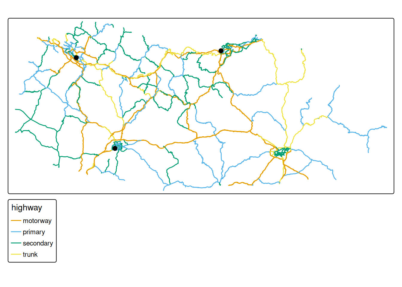
6.2 Calculate network diameter
The diameter tells us the longest shortest-path distance in the network. We calculate it in both travel time and distance.
# Diameter in travel time (minutes)
diam_time <- diameter(
    sf_net_simpl,
    directed = FALSE,
    weights = pull(sf_net_simpl, "travel_time")
)
cat("Network diameter (travel time):", as.numeric(diam_time), "minutes\n")

# Diameter in distance (kilometres)
diam_dist <- diameter(
    sf_net_simpl,
    directed = FALSE,
    weights = pull(sf_net_simpl, "dist")
) *
    1e-3 # Convert from m to km
cat("Network diameter (distance):", diam_dist, "km\n")
6.3 Calculate edge betweenness centrality
Betweenness centrality measures how often a road segment appears on shortest paths between all pairs of nodes. Roads with high centrality are usually key components in the network.
# Calculate edge betweenness centrality weighted by travel time
sf_net_simpl <- sf_net_simpl |>
    activate(edges) |>
    mutate(
        # betweenness: higher values = more central to network connectivity
        betweenness = centrality_edge_betweenness(weights = travel_time)
    )

# Visualise centrality as a map
ggplot() +
    geom_sf(
        data = st_as_sf(sf_net_simpl, "edges"),
        aes(colour = log10(betweenness)),
        linewidth = 1
    ) +
    scale_colour_viridis_c(name = "Log10(Betweenness)") +
    theme_void() +
    labs(title = "Road Network Centrality")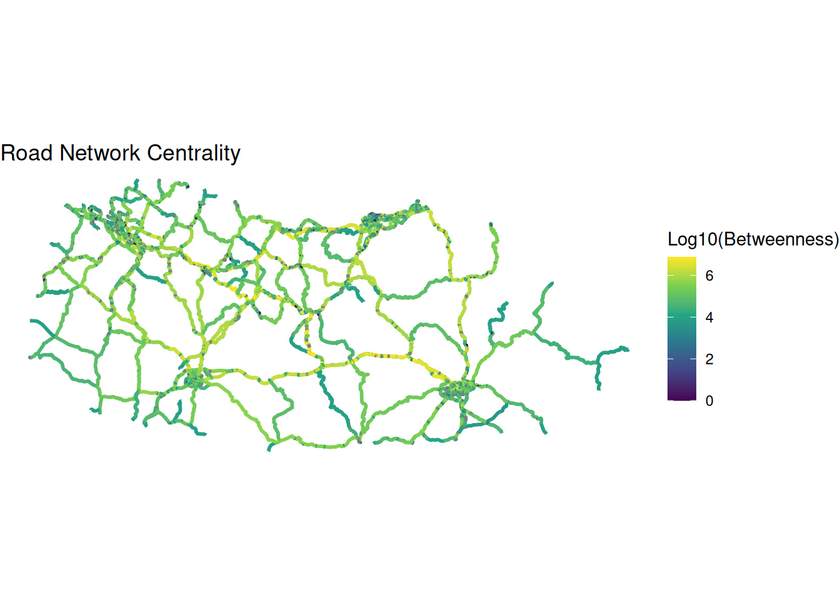
7 Routing and traffic assignment
7.1 Map sample zones to network nodes
To perform routing, we must link our OD zones to the nearest network nodes.
# Extract nodes as spatial features
sf_nodes <- st_as_sf(sf_net_simpl, "nodes")

# Find the nearest node for each sample zone
node_indexes <- sample_zones |>
    st_transform(st_crs(sf_net_simpl)) |>
    st_nearest_feature(sf_nodes)

# Create a lookup table linking zones to nodes
zone_to_node <- tibble(
    zone = sample_zones$id,
    node = node_indexes
)

# Create an origin-destination table
# We'll route from one zone to all others
sample_od <- expand_grid(
    origin = sample_zones$id[2],
    dest = sample_zones$id) |>
    filter(origin != dest) |>
    # Join with node indices
    left_join(zone_to_node, by = c("origin" = "zone")) |>
    left_join(zone_to_node, by = c("dest" = "zone"),
              suffix = c(".o", ".d"))
7.2 Find the peak flow hour
We identify the hour with the highest total flows to use for our routing analysis.
# Aggregate flows by hour and find the peak
max_flow_time <- flows_north_time |>
    semi_join(sample_od,
              by = c("origin","dest")) |>
    summarise(across(count,sum),.by = time) |>
    slice_max(n = 1,order_by = count) |>
    pull(time)

cat("Peak flow hour:", max_flow_time, "\n")
Let’s join the flows to the sample OD pairs
sample_od <- sample_od |>
    # Join with flow data at peak hour
    left_join(
        flows_north_time |>
            filter(time == max_flow_time) |>
            select(-time),
        by = c("origin", "dest")
    )

# Calculate straight-line distance between zones
sample_od$straight_line_dist <- st_distance(
    sample_zones[match(sample_od$origin, sample_zones$id), ],
    sample_zones[match(sample_od$dest, sample_zones$id), ],
    by_element = TRUE
) |>
    as.numeric()
7.3 Calculate shortest paths
We use the Dijkstra algorithm (via st_network_paths()) to find the quickest route between each OD pair, weighted by travel time.
# Calculate quickest paths from one origin to all destinations
# weights = "travel_time" means we minimise travel time, not distance

# This code has been extracted from the sfnetworks documentation and adapted for our dataset

paths <- st_network_paths(
    sf_net_simpl,
    from = sample_od$node.o[1], # Start from first origin
    to = sample_od$node.d, # End at all destinations
    weights = "travel_time"
)

# Helper function to plot a path on the network
plot_path <- function(node_path) {
    sf_net_simpl %>%
        activate("nodes") %>%
        slice(node_path) %>%
        plot(cex = 1.5, lwd = 1.5, add = TRUE)
}

# Set up plot with sample colours
colours <- sf.colors(4, categorical = TRUE)

# Plot the network and overlay all paths
plot(sf_net_simpl, col = "grey")
paths %>%
    pull(node_paths) %>%
    walk(plot_path)

# Highlight sample zones
sf_net_simpl %>%
    activate("nodes") %>%
    st_as_sf() %>%
    slice(node_indexes) %>%
    plot(col = colours, pch = 8, cex = 2, lwd = 2, add = TRUE)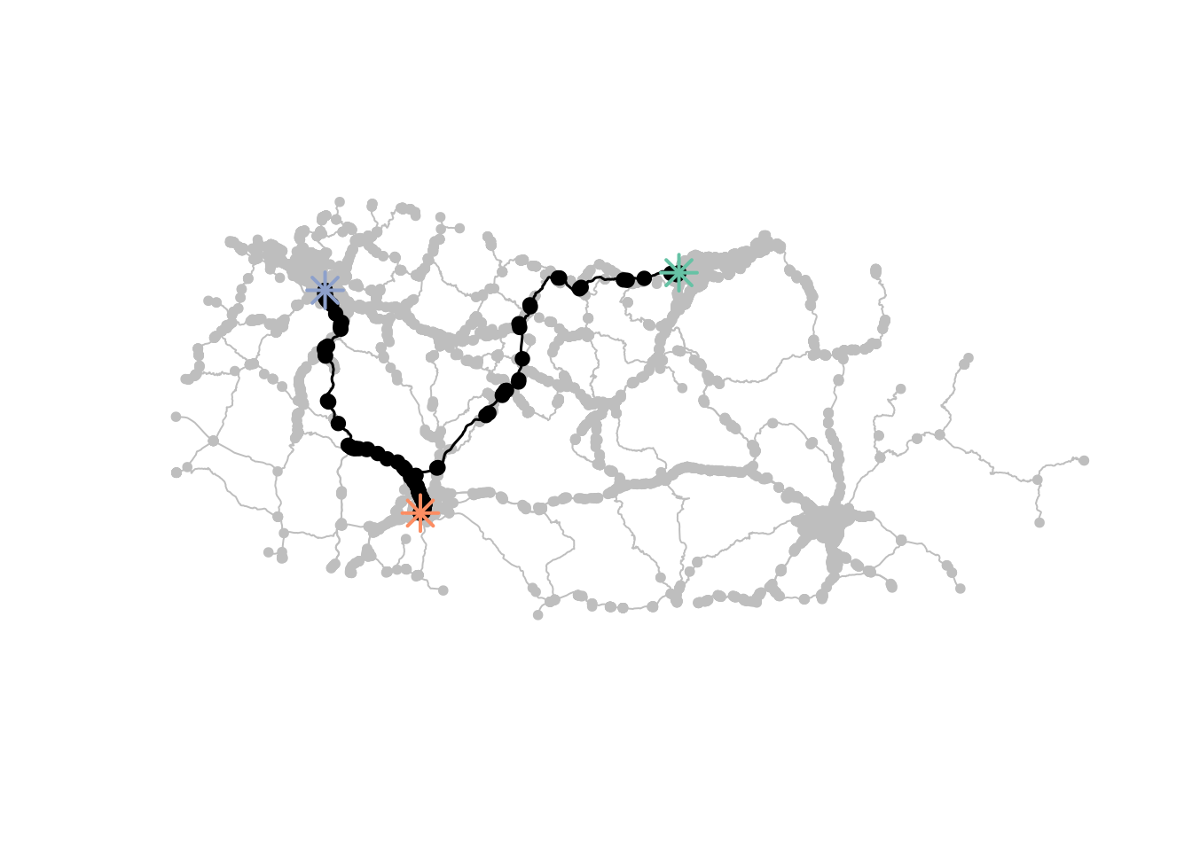
7.4 Extract route characteristics
For each path, we extract the total distance and travel time.
# Extract total distance for each path
sample_od$network_dist <- vapply(
    paths$edge_paths,
    function(edges) {
        pull(sf_net_simpl, "dist")[edges] |> sum()
    },
    numeric(1)
)

# Extract total travel time for each path
sample_od$travel_time <- vapply(
    paths$edge_paths,
    function(edges) {
        pull(sf_net_simpl, "travel_time")[edges] |> sum()
    },
    numeric(1)
)
7.5 Measure route directness
Directness compares the actual route distance to the straight-line distance. A value of 1.0 means the route is perfectly direct; higher values indicate more circuitous routing.
sample_od_summary <- sample_od |>
    mutate(
        directness = straight_line_dist / network_dist,
        # Convert travel time from seconds to minutes
        travel_time_min = as.numeric(travel_time) / 60
    ) |>
    select(
        origin,
        dest,
        straight_line_dist,
        network_dist,
        directness,
        travel_time_min,
        count
    )

# Display a summary
print(sample_od_summary)
8 Assign flows to network
8.1 Apply all-or-nothing traffic assignment
We assign all OD flows to their shortest paths. This creates an estimate of traffic volume on each road segment.
# Extract edges as spatial features
sf_edges <- st_as_sf(sf_net_simpl, "edges")
# Assign flows to edges
# For each OD pair, we add its flow count to all edges in its shortest path
edge_flows <- lapply(
1:nrow(sample_od),
function(i) {
# Get edges for this path
path_edges <- sf_edges[paths$edge_paths[[i]], ] |>
st_drop_geometry()
# Add flow count
path_edges$flow <- sample_od$count[i]
path_edges
}
) |>
bind_rows() |>
# Aggregate flows for each edge (in case multiple paths use the same edge)
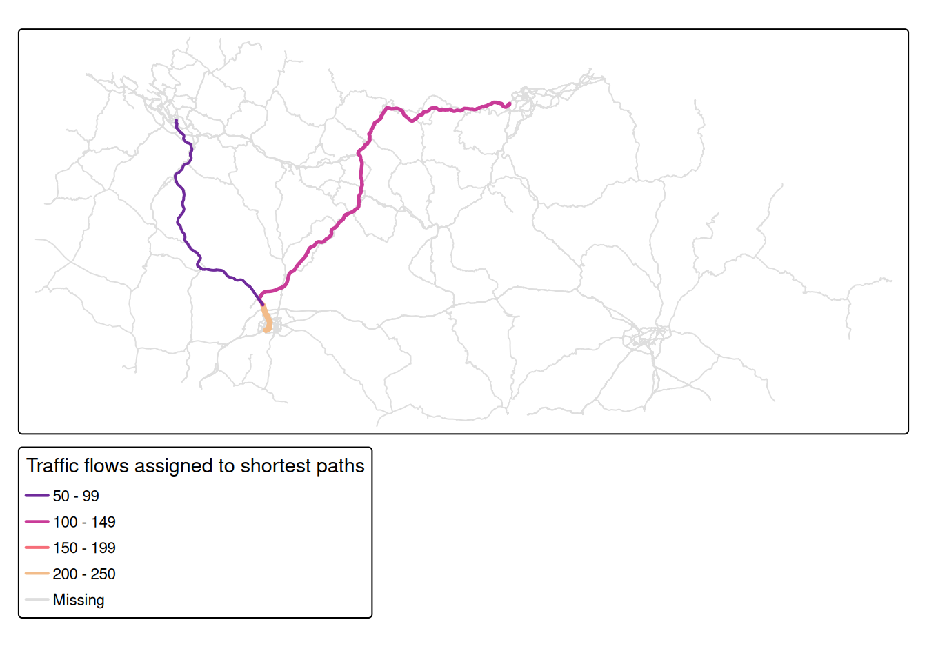
summarise(across(flow, sum), .by = c(from, to))9 Visualise results
9.1 Create a flow map
Finally, we visualise the traffic flows on the network, showing which roads carry the most traffic.
sf_edges |>
    left_join(edge_flows, by = c("from", "to")) |>
    tm_shape() +
    # Colour and width roads by flow volume
    tm_lines(
        col = "flow",
        col.scale = tm_scale_intervals(
            n = 5,
            values = "carto.ag_sunset"
        ),
        col.legend = tm_legend(
            title = "Traffic flows assigned to shortest paths",
            legend.position = c("left", "bottom")),
        lwd = "flow",
        lwd.scale = tm_scale_intervals(
            n = 3,
            values = c(2, 3, 4),
            value.na = 1
        ),
        lwd.legend = tm_legend_hide()
) 
Reuse
Copyright
© 2026 Robin Lovelace, Juan Fonseca, and contributors