Prerequisites
1 Introduction
Welcome to the Mobile Tartu 2026 Transport Data Science workshop! This document outlines the prerequisites for the workshop, and is intended as homework to be completed before the session. If you have any issues completing the prerequisites, please get in touch on github.com/tdscience/tartu26 or by sending the organiser (Robin Lovelace) an email.
There are two main ways to run the workshop materials:
- Local setup on your computer (recommended, see Section 2).
- Cloud-based setup using GitHub Codespaces, Posit Cloud, or similar services (as a backup if you cannot get the software installed locally, see Section 3).
Within each approach, there are various options for software and data setup.
Which to use?
- We recommend the local setup on your own machine so you can run the code directly, learn how to manage the required software, and have everything configured for future use.
- If you run into issues installing the software locally, do not have admin rights to install tools like Docker, or have a machine with limited hardware resources, the cloud-based GitHub Codespaces option serves as an excellent, pre-configured backup that runs entirely in your browser.
Whichever option you choose, ensure you have a good handle on the software and data setup before the workshop to make the most of the session.
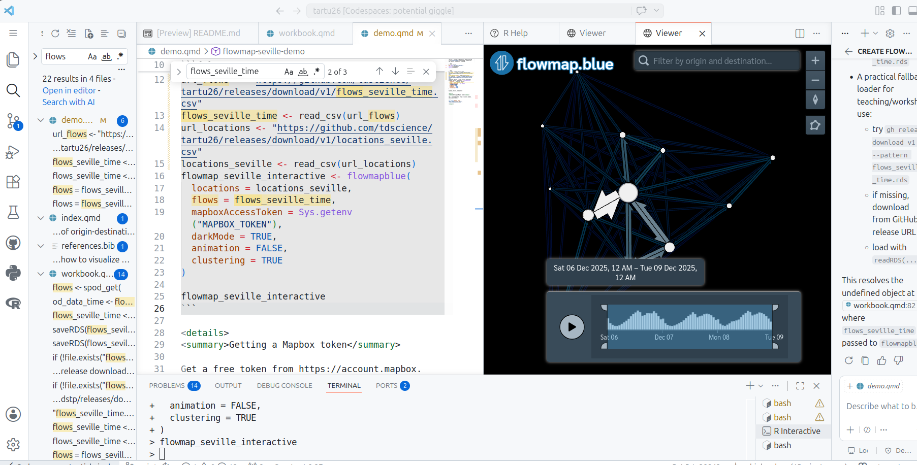
At a minimum, you should be able to reproduce the figure shown at the end of this document, which is an interactive flow map of Seville using the spanishoddata package.
If you’re just curious and want to dive in with minimal set-up, click the link below to fire-up a cloud-based environment to run the code:
![]()
For more information, see the detailed cloud setup instructions in Section 3.
2 Local Setup
If you prefer to run the workshop materials on your own computer, we recommend a machine with a minimum of 16 GB RAM due to the size of the datasets we will be processing.
The workshop materials support both R and Python development paths. You can choose the setup method that best fits your preference:
For local setup, we recommend using the GitHub CLI (gh) to clone the repository and interact with GitHub from your terminal.
gh repo clone tdscience/tartu262.1 Option A: Local devcontainer (recommended if you have admin rights to install Docker)
Click to view setup steps
This is the most reliable way to ensure a consistent environment. The repository includes a pre-configured .devcontainer that sets up all dependencies (R, Python, Quarto, VS Code extensions) inside an isolated container (the same environment used in the cloud-based backup option).
To use this option:
- Ensure you have Docker Desktop and VS Code installed on your machine.
- Install the Dev Containers extension in VS Code.
- Clone the repository and open the folder in VS Code.
- Press
Ctrl+Shift+P(orCmd+Shift+Pon macOS) to open the Command Palette, and select Dev Containers: Reopen in Container.
2.2 Option B: Local R/RStudio installation
Click to view setup steps
If you prefer a native R setup on your machine, please ensure you have the required runtimes, IDE, and tools installed.
2.2.1 Software Requirements
- R (>= 4.3): The language runtime.
- RStudio or Positron: The IDE.
- Quarto CLI: Used to compile and render the workshop documents and workbook.
- Git: Version control software to manage code and download files.
2.2.2 R Packages
Install the necessary packages for the workshop using the pak package (recommended):
install.packages("pak")
pak::pak("tdscience/tartu26")
Alternatively, you can install them manually using:
Manual installation instructions
If you don’t have {pak} installed, you can use install.packages() to install the required packages. Running the following code is equivalent to using pak to install the dependencies:
install.packages(c(
  "tidyverse",
  "sf",
  "tmap",
  "osmdata",
  "spanishoddata",
  "flowmapblue",
  "fs",
  "htmlwidgets"
))
2.3 Option C: Local Python/VS Code installation
Click to view setup steps
If you prefer a native Python setup on your machine, we use a modern, fast conda/mamba alternative package manager called Pixi to quickly install and manage all dependencies.
2.3.1 Software Requirements
- Python (>= 3.10): The language runtime.
- VS Code or Positron: The IDE.
- Quarto CLI: Used to compile and render the workshop documents and workbook.
- Git: Version control software to manage code and download files.
- Pixi: A fast package manager. Follow the Pixi installation instructions for your operating system.
2.3.2 Installing Dependencies and Running Python
Once Pixi is installed, open your terminal in the cloned repository directory. You can initialize the project environment and run Jupyter Lab with:
pixi run jupyter labOr you can use VS Code’s Jupyter extension and select the environment created by Pixi.
We use DuckDB’s Python interface directly to handle and query large transport datasets highly efficiently, as demonstrated in the separate demo-py.qmd file.
2.3.3 Rendering Quarto Documents with Pixi
To render or preview the Quarto files locally using the Python environment managed by Pixi (which contains nbclient and all data science dependencies), prefix your Quarto commands with pixi run:
pixi run quarto render demo-py.qmd
pixi run quarto preview
Alternatively, you can activate the Pixi environment shell first and then run Quarto normally:
pixi shell
quarto render demo-py.qmd
2.4 Data
We will use open datasets throughout the workshop. All required data will be downloadable during the sessions, but you may want to download the larger datasets in advance to save time.
See the releases page for links to the datasets used in the workshop.
You are welcome to bring your own origin-destination and network data if you wish to follow along and implement the concepts with your own datasets. There will be less support for custom datasets. You are encouraged to experiment with your own data after the workshop, and have fun!
3 Cloud Setup (Backup Option)
If you cannot install the required software locally on your computer, the cloud-based option allows you to run the complete workshop environment entirely in your web browser using GitHub Codespaces.
3.1 GitHub
To use GitHub Codespaces or access repository resources, you must have a GitHub account. Go to GitHub and sign-up if you haven’t already done so.
If you are a student, researcher, or teacher at an accredited academic institution, you can sign up for the GitHub Global Campus program to get free premium benefits:
- GitHub Pro: Upgraded account limits, including more GitHub Codespaces hours and storage (ideal for running data-intensive environments like this workshop).
- GitHub Copilot: Free access to GitHub’s AI developer tool to write code, debug, and learn faster.
- Developer Packs: Free access to top-tier developer tools, cloud hosting credits, and subscriptions.
You can apply with your academic email address or school ID at education.github.com.
After you have a GitHub account, you can launch the workspace in GitHub Codespaces by clicking the badge below. Note: it takes around 5 minutes to set up the Codespace environment, so be patient, read-up on some of the links in this website, or get a coffee!
![]()
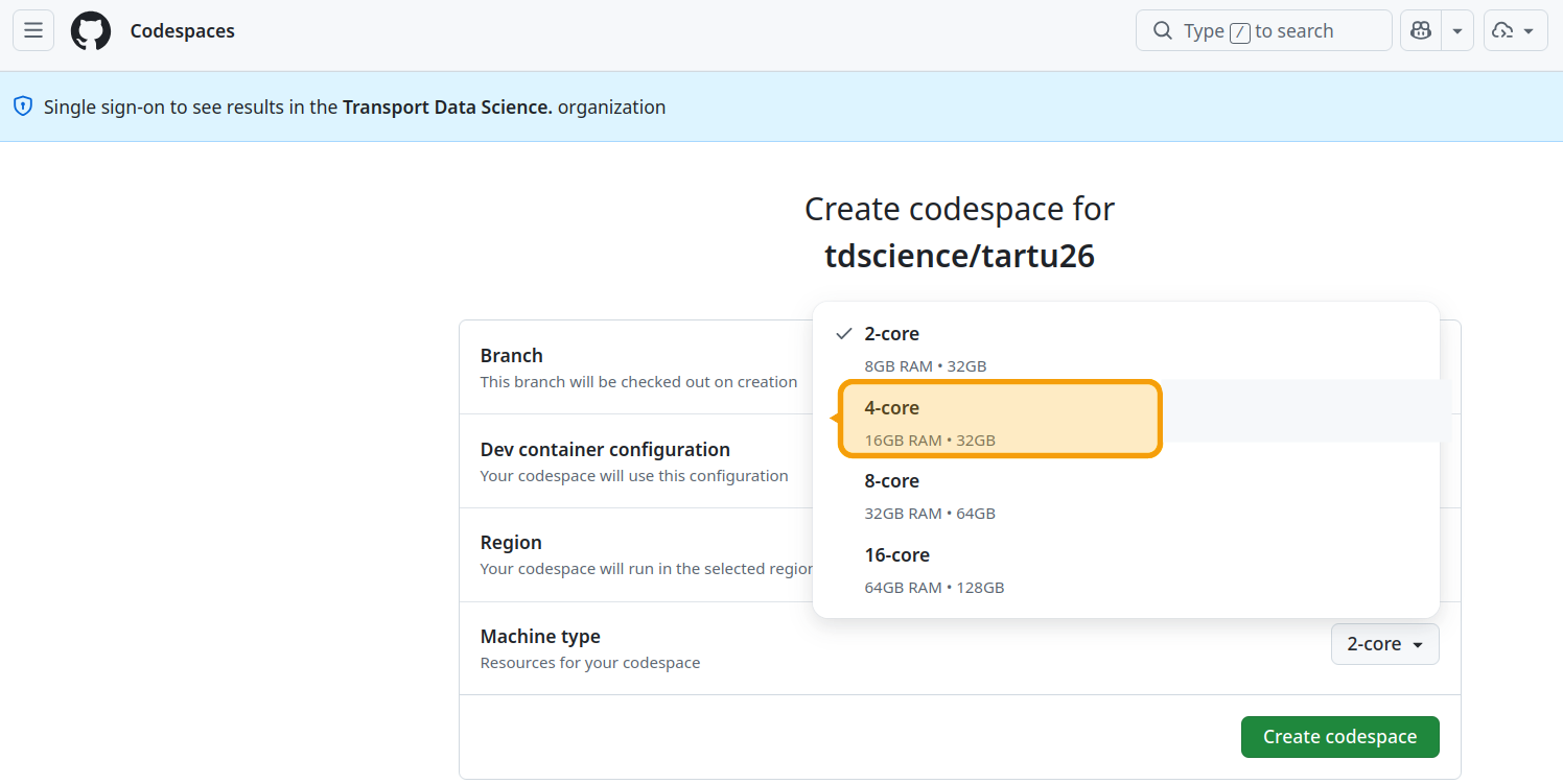
When you click on that button, assuming you’re signed in and do not have any existing codespaces associated with the repo already running, you should see a page with default settings for the codespace. You can leave them all as is except for machine type.
We will be handling a lot of data so select the 4-core option. This gives you 16 GB RAM on a machine with 60 hours of free use per month. That should be plenty for processing the datasets we’ll using in this tutorial. Go for a larger option if you want to import larger datasets but be warned that your compute credits will burn down quicker the larger the machine you’re on, as described in the GitHub Codespaces pricing docs.
About GitHub
While you wait for that to load, it’s worth learning a bit about what GitHub is: it’s the world’s number one platform for hosting and collaborating on code, especially for international and open-source projects, although you can easily host ‘private repos’ also, allowing you to choose who can see and collaborate on your work. Key concepts in GitHub include:
- Repositories, also called repos. These are like folders for your projects, where you can store code, data, and documentation. The workshop materials are hosted in a GitHub repository. See the GitHub repository for the workshop at github.com/tdscience/tartu26 for more details.
- Issues. These are like to-do lists or bug trackers for your code. You can use them to keep track of tasks, bugs, or feature requests for your projects. See the Issues tab in the workshop repository and open a test issue if you want to practice, it’s a great way to communicate, learn, get feedback and collaborate with others.
- Pull requests. These are like proposals for changes to your code. You can use them to suggest changes, review code, and merge changes into your projects. See the Pull Requests tab in the workshop repository for more details. Bonus: open a PR making a change to the README file, it’s a great way to practice and learn about how PRs work (see the GitHub documentation on pull requests for more details).
- Commits. These are like snapshots of your code at a given point in time.
- Branches. These are like different versions of your code that you can work on separately and then merge together.
You can run the code in any GitHub repo in Codespaces by clicking on the green “Code” button and selecting “Open with Codespaces”, as described in the GitHub documentation and shown below. Try to see the options in the green “Code” button for the workshop repository, and try cloning locally or downloading the zip file to see the different options available as a bonus. The “Codespaces” option is the one to launch the cloud-based environment for the workshop, while the “Download ZIP” option allows you to download the repository files to your local machine without using Git.
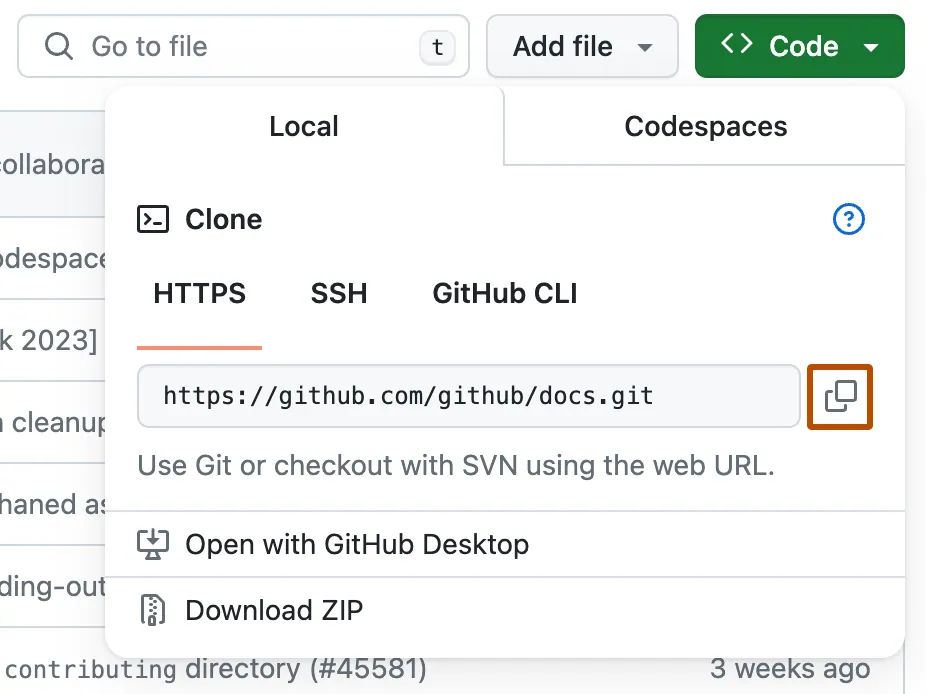
The “Local” clone — with HTTPS, ssh or GitHub CLI options — are for cloning the repository to your local machine, which is not required if you are using Codespaces, but may be useful if you want to work on the materials locally, as described in Section 2.
After the Codespace has finished ‘spinning-up’, you will see something like this:
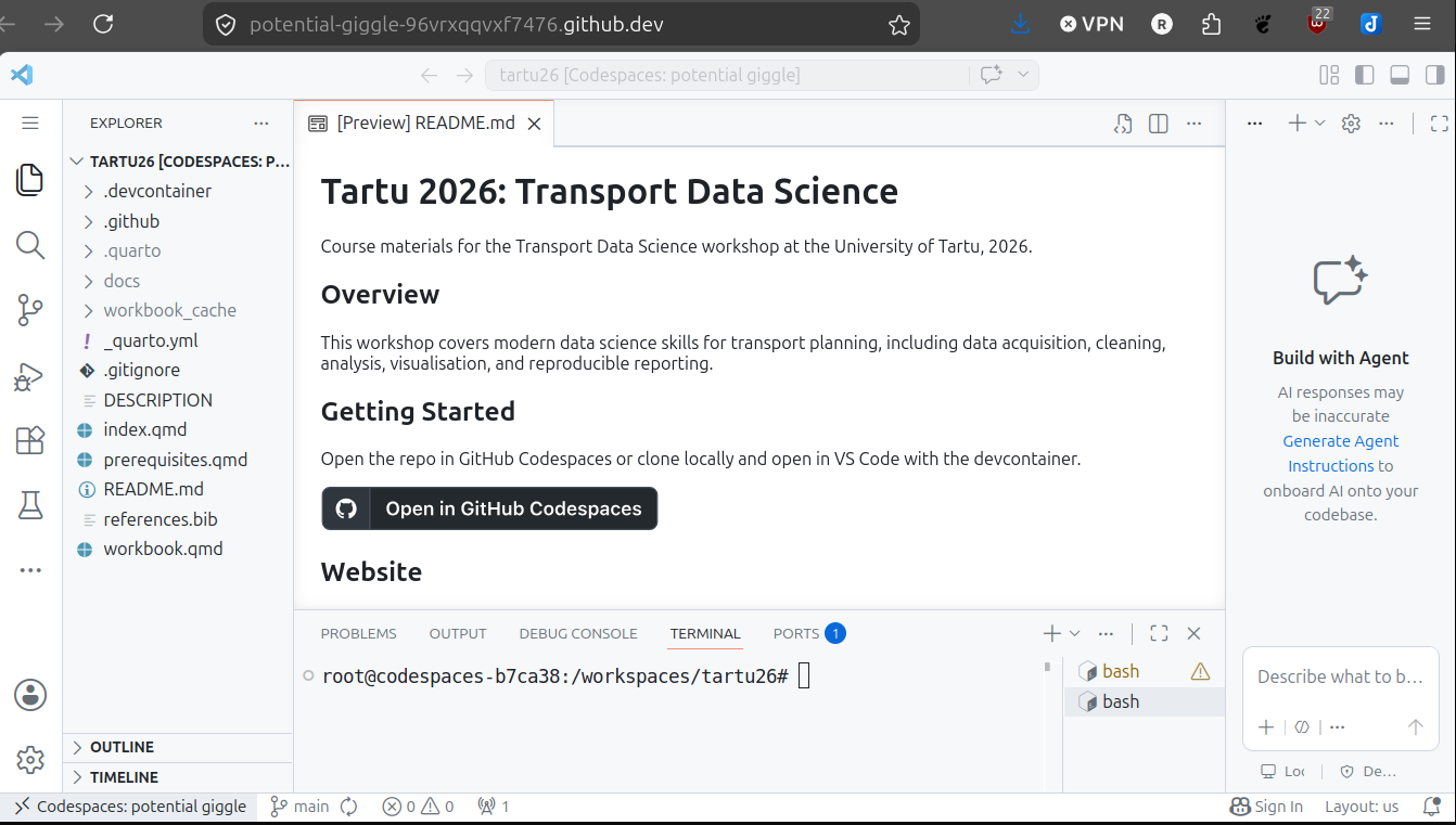
There are a few things worth noting about the Codespace environment shown above:
- The repository files are visible in the Explorer pane on the left (including
.devcontainer, Quarto files, and workshop documents), confirming that the workspace has loaded correctly. - The editor opens files directly in the browser-based VS Code interface. In the screenshot,
README.mdis shown in preview mode. - The integrated terminal at the bottom is ready to run commands in the project directory (
/workspaces/tartu26). This is where you can run workshop code and render Quarto documents. - If your environment took around 5 minutes to start, this is expected for first launch: once loaded, you can proceed with the exercises normally.
- You have a unique Codespace URL (e.g.
https://tdscience-tartu26-abc123-xyz456.codespaces.github.com) that you can bookmark and return to later, and share with others if you want to collaborate.
From that point, you’re almost ready to start writing and running code for the workshop! It’s worth being aware of a few different ways to run code interactively in the Codespace environment.
To check that the code runs for this tutorial, open the demo.qmd file in the editor and run the code chunks interactively using Ctrl+Enter (or Cmd+Enter on Mac) to execute the code line-by-line.
If it worked it should look something like this:
Congratulations if so, you have completed the prerequisites for the workshop and are ready to start learning about transport data science with R and Python!
Other cloud-based environments
Other cloud services are available. One that is well-suited for data science is Posit Cloud, but unfortunately has a maximum session RAM use of only 1GB, which is not enough for the datasets we’ll be using in this workshop. For these cloud services, you may still need to install the required packages the first time you launch a new session (see the R Packages section).4 The outcome: an interactive flow map of Seville
After running the code shown below, from demo.qmd, you should see an interactive flow map of Seville in the Viewer pane of your IDE.
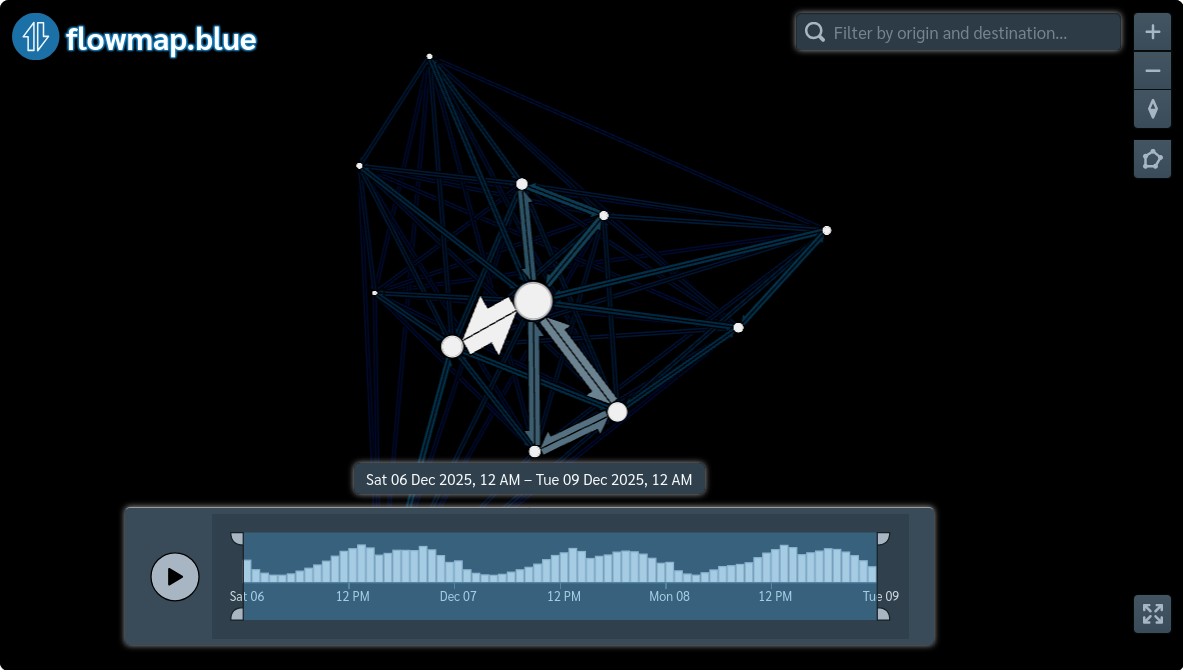
See an interactive version of the map by downloading and then releasing the seville_flowmap_embed.html file from the github.com/tdscience/tartu26/releases page.