# This code chunk creates an interactive flow map for Seville,
# demonstrating animation and time-filtering capabilities.
# It is based on the vignette from the rOpenSpain/spanishoddata package.

# --- 1. Load necessary libraries ---
library(spanishoddata)
library(flowmapblue)
library(tidyverse)
library(sf)

# --- 2. Set up Mapbox Access Token (required for the basemap) ---
# Get a free token from https://account.mapbox.com/access-tokens/
# Sys.setenv(MAPBOX_TOKEN = "YOUR_MAPBOX_ACCESS_TOKEN")
# Or, longer term solution: usethis::edit_r_environ()
# Restart R after setting the token for it to take effect

# --- 3. Download and prepare the data ---

# Get OD data for the most recently days
zones <- spod_get_zones(zones = "distr", ver = 2)
valid_dates <- spod_get_valid_dates(2)
recent_dates = tail(valid_dates, 3)

# Identify zones corresponding to Seville
zones_seville <- zones |>
  filter(grepl("^Sevilla distrito", name, ignore.case = TRUE))
mapview::mapview(zones_seville)

# Create a 10km buffer to define the Functional Urban Area (FUA)
zones_seville_fua <- zones[st_buffer(zones_seville, dist = 10000), ]
plot(st_geometry(zones_seville_fua))

# Prepare the location data (centroids) for the flow map
sf::sf_use_s2(FALSE)
locations_seville <- zones_seville_fua |>
  st_transform(crs = 4326) |>
  st_centroid() |>
  st_coordinates() |>
  as.data.frame() |>
  mutate(id = zones_seville_fua$id) |>
  rename(lon = X, lat = Y)

# # Uncomment to re-download the data:
# flows <- spod_get(
#   type = "origin-destination",
#   zones = "districts",
#   dates = recent_dates
# )

# # Process the OD data to create a timestamp for each flow
# od_data_time <- flows |>
#   mutate(time = as.POSIXct(paste0(date, "T", hour, ":00:00"))) |>
#   group_by(origin = id_origin, dest = id_destination, time) |>
#   summarise(count = sum(n_trips, na.rm = TRUE), .groups = "drop") |>
#   collect()
# saveRDS(od_data_time, "od_data_time.rds")
# fs::file_size("od_data_time.rds")
# # --- 5. Filter data for the Seville region ---

# # Filter the time-based OD data to include only flows within the Seville FUA
# flows_seville_time <- od_data_time |>
#   filter(origin %in% zones_seville_fua$id & dest %in% zones_seville_fua$id)
# saveRDS(flows_seville_time, "flows_seville_time.rds")
# fs::file_size("flows_seville_time.rds")
# system("gh release upload v1 flows_seville_time.rds")

# Get that file with:
if(!file.exists("flows_seville_time.rds")) {
  # if you have the gh tool:
  system("gh release download v1 --pattern flows_seville_time.rds")
  download.file("https://github.com/tdscience/dstp/releases/download/v1/flows_seville_time.rds", "flows_seville_time.rds")
  flows_seville_time <- readRDS("flows_seville_time.rds")
}


# --- 6. Generate the interactive flow map ---

# Create the plot with animation and clustering enabled.
# The resulting map will have a time slider to filter flows by hour.
flowmap_seville_interactive <- flowmapblue(
  locations = locations_seville,
  flows = flows_seville_time,
  mapboxAccessToken = Sys.getenv("MAPBOX_TOKEN"),
  darkMode = TRUE,
  animation = FALSE,
  clustering = TRUE
)

# Display the map
flowmap_seville_interactive
# Save the map as an HTML file
htmlwidgets::saveWidget(flowmap_seville_interactive, "seville_flowmap.html")
system("firefox seville_flowmap.html")
fs::file_size("seville_flowmap.html")
system("gh release create")
system("gh release upload v1 seville_flowmap.html")Spatio-temporal data
1 Spatio-temporal data with OD data
This exercise is based on the tutorial “Analysing massive open human mobility data in R using spanishoddata, duckdb and flowmaps” by Egor Kotov [@kotov2025].
This is a more advanced exercise that benefits from having a fast internet connection, decent compute resources, and an interest in the Iberian Peninsula.
1.1 Practical 4 options
There are four options for this practical session:
Get stuck-into open access CDR (call detail records) data from Spain using the
spanishoddatapackage (detailed below with example for Seville)Revisit the London Cycle Hire data from session 3 and visualize flows using the
flowmapbluepackageExplore changes in the spatial and temporal distributions of road traffic collisions using the
stats19packageBring your own data (BYOD)!
The spanishoddata option is based on the tutorial “Analysing massive open human mobility data in R using spanishoddata, duckdb and flowmaps” by Egor Kotov [@kotov2025].
See ekotov.pro for details:
- Setting up the software
- Importing the data
- Visualising the data with flowmaps An example of code using the package is shown below, which results in an interactive flow map for Seville, as shown below and in the interactive HTML file seville_flowmap.html in the releases section of this repository.
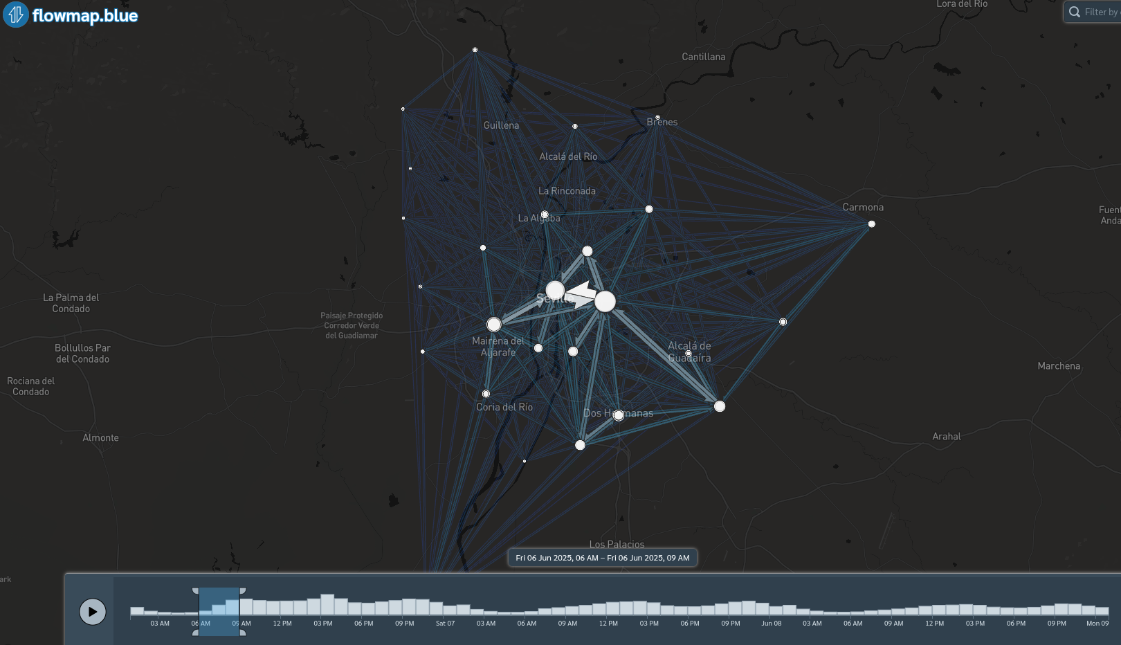
1.2 spanishoddata
Download a load of data from Spain!
![]()
1.3 Option 2: London Cycle Hire flow visualization
To extend the analysis from session 3, prepare the cycle hire data as origin-destination flows with timestamps (e.g., from start/end stations and times). Then use flowmapblue for interactive visualization.
See the flowmapblue vignette for details.
# Load libraries (assuming data prepared as in s3.qmd)
library(flowmapblue)
library(tidyverse)
library(sf)

# Assume 'cycle_data' is loaded with columns: origin_id, dest_id, time (POSIXct), count
# And 'stations' sf with id, lon, lat

# Prepare locations (stations)
locations_london <- stations |>
  st_transform(crs = 4326) |>
  st_coordinates() |>
  as.data.frame() |>
  mutate(id = stations$id) |>
  rename(lon = X, lat = Y)

# Prepare flows (aggregate if needed)
flows_london <- cycle_data |>
  group_by(origin = origin_id, dest = dest_id, time) |>
  summarise(count = n(), .groups = "drop")  # or sum trips

# Create interactive flow map
flowmap_london <- flowmapblue(
  locations = locations_london,
  flows = flows_london,
  mapboxAccessToken = Sys.getenv("MAPBOX_TOKEN"),
  animation = TRUE,
  clustering = TRUE
)

flowmap_london

# Save
htmlwidgets::saveWidget(flowmap_london, "london_flowmap.html")
1.4 Option 3: Road traffic collisions with stats19
The stats19 package provides access to detailed road safety data for Great Britain, including timestamps and locations for spatio-temporal analysis.
library(stats19)
library(tidyverse)
library(lubridate)

# Download collisions for 2020 (pandemic year) and 2021
collisions_20 <- get_stats19(year = 2020, type = "collision", ask = FALSE)
collisions_21 <- get_stats19(year = 2021, type = "collision", ask = FALSE)

# Format to sf (for spatial if needed)
london_20 <- format_sf(collisions_20)
london_21 <- format_sf(collisions_21)

# Temporal analysis: extract hour and compare distributions
london_20 <- london_20 |>
  mutate(
    date_time = as.POSIXct(datetime, tz = "Europe/London"),
    hour = hour(date_time),
    year = 2020
  )

london_21 <- london_21 |>
  mutate(
    date_time = as.POSIXct(datetime, tz = "Europe/London"),
    hour = hour(date_time),
    year = 2021
  )

# Combine and plot hourly distribution
temporal_changes <- bind_rows(london_20, london_21) |>
  filter(longitude > -0.5, longitude < 0.25, latitude > 51.28, latitude < 51.72)  # rough London bbox

ggplot(temporal_changes, aes(x = hour, fill = factor(year))) +
  geom_histogram(binwidth = 1, position = "dodge", alpha = 0.7) +
  labs(title = "Hourly distribution of road collisions in London: 2020 vs 2021",
       x = "Hour of day", y = "Number of collisions",
       fill = "Year") +
  theme_minimal()

# For spatial: map collisions by hour or severity
# tmap::tm_shape(london_20) + tmap::tm_dots(col = "hour")
For spatial analysis, filter to your area of interest and use tmap or ggplot with sf. See stats19 articles for more.
1.5 Option 4: Bring your own data (BYOD)
If you have access to your own spatio-temporal transport data (e.g., GPS trajectories, sensor data, or time-stamped OD matrices):
- Load and clean the data in R (use
readr,sf,lubridatefor timestamps). - Aggregate into flows: origin, destination, time, count.
- Visualize: use
flowmapbluefor interactive maps,ggplot2+geom_sffor static plots, orleafletfor web maps. - Analyze: explore temporal patterns with
tsibbleorlubridate, spatial withsf.
Share your results or challenges in the discussion!
Reuse
Copyright
© 2025 Robin Lovelace