options(repos = c(CRAN = "https://cloud.r-project.org"))
if (!require("pak")) install.packages("pak")
pkgs = c(
    "sf",
    "tidyverse",
    "tmap",
    "stats19",
    "stplanr",
    "osmextract",
    "zonebuilder"
)
pak::pak(pkgs)
library(tidyverse)
zones = zonebuilder::zb_zone("Leeds", n_circles = 3)
study_area = zones |>
  sf::st_union()
extra_tags = c(
  "maxspeed",
  "lit",
  "cycleway"
)
osm_network = osmextract::oe_get(
  place = study_area,
  boundary = study_area,
  boundary_type = "clipsrc",
  extra_tags = extra_tags
)Prerequisites
1 Course Prerequisites
This course assumes working knowledge with R or Python for research. We assume that you are already comfortable with an integrated development environment (IDE), such as RStudio or VS Code. You must have a GitHub account and it will be beneficial to be familiar with the concepts of version control, although we will cover these in the course.
Familiarity with referencing software such as Zotero (recommended) and bibliography file formats such as BibTeX will be beneficial, but not essential.
2 Software Prerequisites
You should bring a laptop with the following software installed and tested to check it works:
- Quarto (minimum version: 1.5.45)
- A tested R or Python installation or both (note: if you have Docker installed you should be able to run R and Python inside a devcontainer, works best with VS Code)
- RStudio or VS Code IDE
- If you use RStudio, it should ‘just work’ with R and Quarto.
- If you will use VS Code for the course, you need the following extensions:
- The R extension
reditorsupport.rif using R - The Python extension
ms-python.pythonif using Python - The quarto extention
quarto.quarto
- The R extension
- For experienced users: you can also use an IDE of your choice, for example Positron IDE which is based on VS Code and has R, Python and Quarto support built-in.
- Git, installed with one of the following packages:
- GitHub Desktop (see desktop.github.com)
- Git for the command line (see git-scm.com)
- The
ghcommand-line tool (see cli.github.com for installation and set-up instructions)
3 Recommended Online Courses
Students should take these short but very useful online courses to prepare:
- Intro to GitHub (should take less than an hour)
- Communicate using Markdown (should take around 30 minutes or less)
4 Testing your setup
You can test your setup by running the following code in R or Python.
osm_network |>
  select(maxspeed) |>
  plot()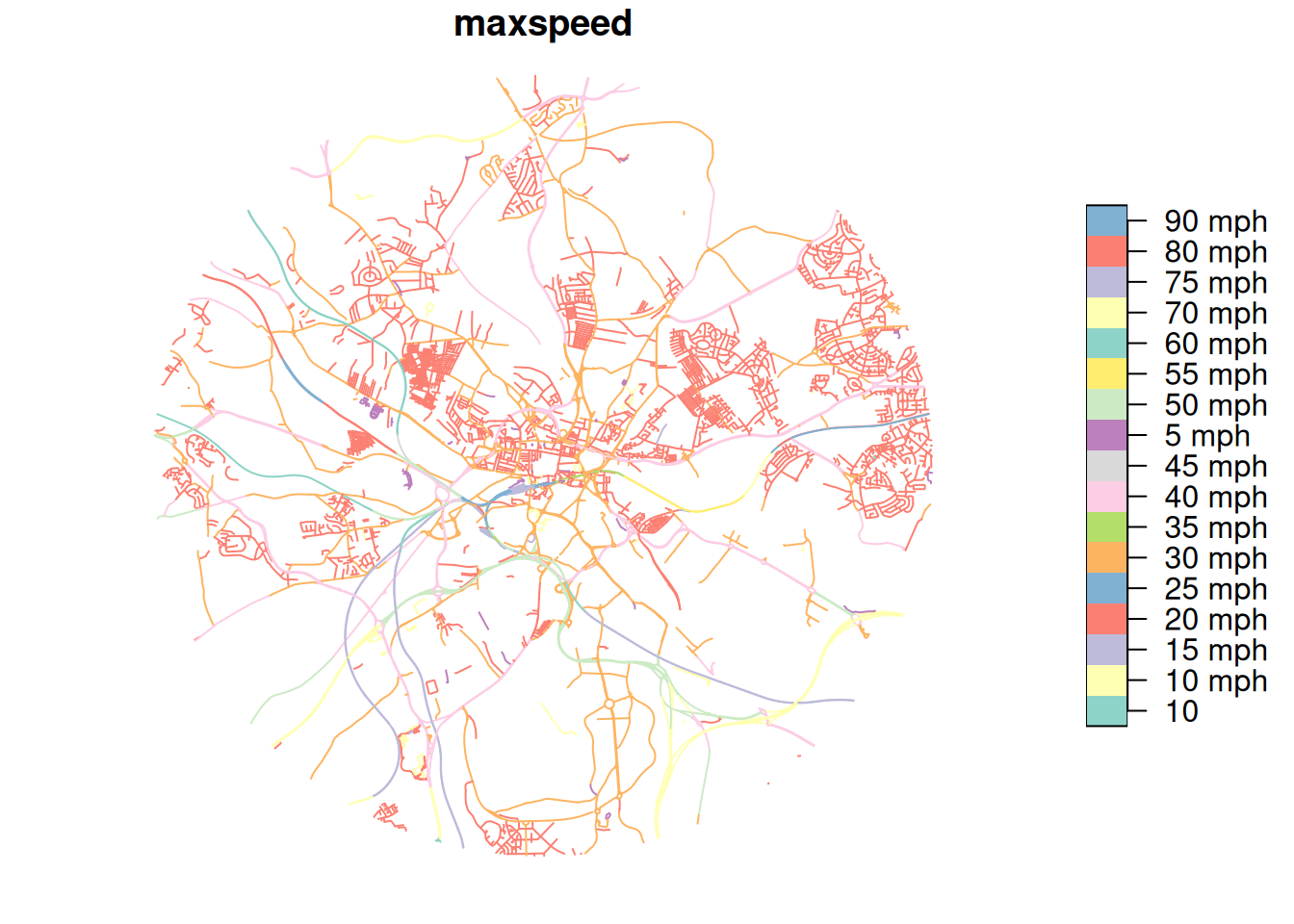
sf::write_sf(study_area, "leeds_study_area.geojson")import osmnx as ox
import geopandas as gpd
import matplotlib.pyplot as plt
import shapely
study_point = shapely.Point(-1.55, 53.80) # Latitude and Longitude for Leeds
study_geom = gpd.GeoSeries([study_point], crs=4326)
study_polygon = study_geom.to_crs(epsg=3857).buffer(6000).to_crs(epsg=4326).unary_union
study_polygon_gpd = gpd.GeoDataFrame(geometry=[study_polygon], crs="EPSG:4326")
# Read-in geojson already saved from R
study_polygon = gpd.read_file("leeds_study_area.geojson")
# study_polygon_gpd.explore()
tags = {"highway": True, "maxspeed": True, "lit": True, "cycleway": True}
gdf = ox.features_from_polygon(study_polygon, tags)
gdf = gdf[gdf.geom_type.isin(["LineString", "MultiLineString"])]
gdf = gdf.to_crs(epsg=3857)
gdf.plot(column="maxspeed", figsize=(10, 10), legend=True)
plt.show()Let us know how you get on and let us know if you have any issues getting set up, either by email, or (preferably) via the Discussion forum on GitHub associated with this course repository at github.com/tdscience/dstp/discussions.
Reuse
Copyright
© 2025 Robin Lovelace