Routing and route network analysis

1 Introduction

This session demonstrates routing and network analysis techniques. By the end of this session, you should be able to:

• Understand the principles of routing and network analysis
• Use routing services such as OpenTripPlanner for multi-modal routing
• Create and analyze route networks
• Apply network centrality measures

2 Prerequisites

if (!require("pak")) install.packages("pak")
pak::pkg_install(c("sf", "tidyverse", "stplanr", "dodgr", "opentripplanner", "tmap", "osmextract", "lwgeom"))

library(sf)
library(tidyverse)
library(stplanr)
library(dodgr)
library(opentripplanner)
library(tmap)
library(osmextract)
library(lwgeom)
tmap_mode("view")

3 OpenTripPlanner Routing

OpenTripPlanner (OTP) is a powerful open-source routing engine that supports multi-modal transportation planning.

3.1 Connecting to OTP

otpcon = otp_connect(
  hostname = "otp.robinlovelace.net",
  ssl = TRUE,
  port = 443,
  router = "west-yorkshire"
)

3.2 Basic Routing

# Create a simple walking route from ITS Leeds to Leeds Railway Station
from = stplanr::geo_code("Institute for Transport Studies, Leeds")
to = stplanr::geo_code("Leeds Railway Station")

route_walk = otp_plan(
  otpcon = otpcon,
  fromPlace = from, # c(-1.555, 53.810), # Longitude, Latitude
  toPlace = to, # c(-1.54710, 53.79519),
  mode = "WALK"
)
qtm(route_walk)

You should see something like this, a good route from ITS to the train station. Zoom into the interactive map at leeds_walk_route.html in the releases to see if it’s the same route you would take.

Note

You can download and view the resulting map with the following code:

download.file("https://github.com/tdscience/dstp/releases/download/v1/leeds_walk_route.html")
browseURL("leeds_walk_route.html", browser = "firefox")

Tip

Share the dataset with others as follows:

sf::write_sf(route_walk, "leeds_walk_route.geojson")

3.3 Multi-Modal Routing

# Public transport route
route_transit = otp_plan(
  otpcon = otpcon,
  fromPlace = c(-1.55555, 53.81005),
  toPlace = c(-1.54710, 53.79519),
  mode = c("WALK", "TRANSIT")
)

# Cycling with public transport
route_bike_transit = otp_plan(
  otpcon = otpcon,
  fromPlace = c(-1.55555, 53.81005),
  toPlace = c(-1.54710, 53.79519),
  mode = c("BICYCLE", "TRANSIT")
)

4 Working with Desire Lines

Desire lines represent travel demand between origin-destination pairs.

4.1 Loading OD Data

We’ll import and apply basic preprocessing steps to desire lines from the National Trip End Model (NTEM). Note that we keep the raw data unchanged for reproducibility.

# Load desire lines data
desire_lines_raw = read_sf("https://github.com/ITSLeeds/TDS/releases/download/22/NTEM_flow.geojson")
desire_lines = desire_lines_raw |>
  select(from, to, all, walk, drive, cycle)

# Load zone centroids
centroids = read_sf("https://github.com/ITSLeeds/TDS/releases/download/22/NTEM_cents.geojson")

We’ll also create a smaller subset of the desire lines for demonstration purposes.

## Filter for top 5 desire lines by total trips
desire_top = desire_lines |>
  slice_max(order_by = all, n = 5)

4.2 Visualizing Desire Lines

tm_shape(desire_lines) +
  tm_lines(
    col = "all",
    lwd = "all",
    lwd.scale = tm_scale_continuous(values.scale = 10),
    col.scale = tm_scale_continuous(values = "-viridis")
  ) +
  tm_shape(centroids) +
  tm_dots(fill = "red", size = 0.5)

Extract start and end points as follows:

# Extract start and end points
fromPlace = sf::st_sf(
  data.frame(id = desire_top$from),
  geometry = lwgeom::st_startpoint(desire_top)
)
toPlace = sf::st_sf(
  data.frame(id = desire_top$to),
  geometry = lwgeom::st_endpoint(desire_top)
)

4.3 Calculating Routes

# Calculate driving routes for top desire lines
routes_drive_top = otp_plan(
  otpcon = otpcon,
  fromPlace = fromPlace,
  toPlace = toPlace,
  fromID = fromPlace$id,
  toID = toPlace$id,
  mode = "CAR"
)

4.4 Visualizing Routes

tm_shape(routes_drive_top) +
  tm_lines(col = "blue", lwd = 3)

5 Route Network Analysis

Route networks aggregate individual routes to show cumulative traffic flow.

5.1 Joining routes to create a route network

The full dataset can be loaded as follows:

# Load more comprehensive route data
routes_drive = read_sf("https://github.com/ITSLeeds/TDS/releases/download/22/routes_drive.geojson")
routes_transit = read_sf("https://github.com/ITSLeeds/TDS/releases/download/22/routes_transit.geojson")
# Check the dimensions of these datasets
names(desire_lines)
dim(desire_lines)
names(routes_drive)
dim(routes_drive)
dim(routes_transit)

We’ll join this with the desire lines data to get trip counts associated with each route.

routes_drive_joined = dplyr::left_join(
  routes_drive |>
    rename(from = fromPlace, to = toPlace),
  desire_lines |>
    sf::st_drop_geometry()
)

routes_transit_joined = dplyr::left_join(
  routes_transit |>
    rename(from = fromPlace, to = toPlace),
  desire_lines |>
    sf::st_drop_geometry()
)

5.2 Aggregating Routes

# Create route network by aggregating overlapping routes
rnet_drive = overline(routes_drive_joined, "drive")
tm_shape(rnet_drive) +
  tm_lines(
    col = "drive",
    col.scale = tm_scale_intervals(values = "-viridis", style = "jenks"),
    lwd = 2
  )

5.3 Visualizing Route Networks

tm_shape(rnet_drive) +
  tm_lines(
    col = "drive",
    col.scale = tm_scale_intervals(values = "-viridis", style = "jenks"),
    lwd = 2
  )

6 Bonus: Network Centrality Analysis

Network centrality measures help identify critical infrastructure.

6.1 Preparing Network Data

zones = zonebuilder::zb_zone("Leeds", n_circles = 3)
study_area = zones |>
  sf::st_union()
extra_tags = c(
  "maxspeed",
  "lit",
  "cycleway"
)
roads = osmextract::oe_get_network(
  mode= "driving",
  place = study_area,
  boundary = study_area,
  boundary_type = "clipsrc",
  extra_tags = extra_tags
)

# Filter for main roads
roads = roads |>
  filter(!is.na(highway)) |>
  filter(highway %in% c("primary", "secondary", "tertiary", "residential", "unclassified")) |>
  sf::st_cast("LINESTRING") 

# Create network graph
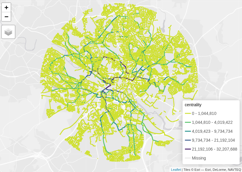
graph = weight_streetnet(roads)

6.2 Calculating and visualising centrality

# Deduplicate edges:
graph = dodgr_deduplicate_graph(graph)
# Calculate betweenness centrality
centrality = dodgr_centrality(graph)
# Convert back to spatial format
centrality_sf = dodgr_to_sf(centrality)

tm_shape(centrality_sf) +
  tm_lines(
    col = "centrality",
    col.scale = tm_scale_intervals(values = "-viridis", style = "fisher"),
    lwd = 3
  )

For large-scale routing on local networks, including traffic impacts, consider the cppRouting package [@larmet2019], which provides efficient C++-based algorithms for shortest paths and traffic assignment. See the repository for examples.

You should get something that looks like this:

Note: you can save an interactive version of the map with tmap_save() and then share it, e.g. with gh release upload to share it on GitHub.

7 Exercise 1: Basic Routing

1. Connect to the OpenTripPlanner server
2. Calculate a walking route between two points in Leeds
3. Visualize the route on a map

# Your code here

8 Exercise 2: Multi-Modal Routing

1. Calculate routes using different modes (walk, transit, bicycle+transit)
2. Compare the travel times and distances
3. Visualize the different route options

# Your code here

9 Exercise 3: Desire Lines Analysis

1. Load the desire lines dataset
2. Filter for the top 5 desire lines by total trips
3. Create a map showing the desire lines colored by mode share

## Your code here

10 Exercise 4: Route Network Creation

1. Load route data for a specific mode with osmextract::oe_get_network() (hint: run ?oe_get_network to find out which modes are available), the osmnx Python package, or any other source
2. Assign values to links and visualise the route network
3. Compare the route network visualization with individual routes

## Your code here

11 Exercise 5: Network Centrality

1. Download road network data for a small area
2. Calculate betweenness centrality
3. Identify the most critical roads in the network

# Your code here

12 Exercise 6: Advanced Routing

• Read over the routing engine setup example and (as a bonus) try to set up your own instance of OpenTripPlanner using Java or Docker.

13 Exercise 7: Vehicle routing with traffic (azuremapsr)

One of the main limitations of routing services is related to the availability of actual traffic data. Services such as Google Maps or Azure provide routing with real-time and historic traffic data.

You can access to those services through some R packages like mapsapi and azuremapsr.

Important

To use any of this services you will need to have an API key for each one. Both packages have instructions for obtaining one in their documentation.

14 Exercise 8: Vehicle routing with traffic (Google)

Use the mapsapi package to interface with the Google Maps Directions API for routing with traffic data. This exercise reproduces the walking route from earlier using the existing from and to objects, then extends to driving with real-time traffic.

Important

You need a Google Maps API key with Directions API enabled. See the mapsapi vignette for setup instructions. Store it as key = readLines("path/to/your/key") or set as environment variable Sys.setenv(GOOGLE_MAPS_API_KEY = "your_key").

1. Load the mapsapi package and use mp_directions to get a walking route.

library(mapsapi)

# Assume 'from' and 'to' are already defined as sf points (from earlier in the session)
# from = stplanr::geo_code("Institute for Transport Studies, Leeds")
# to = stplanr::geo_code("Leeds Railway Station")

# Get walking directions (reproducing the OTP route)
doc_walk = mp_directions(
  origin = from,
  destination = to,
  mode = "walking",
  key = key  # your API key
)

# Extract route as sf lines
route_walk_gmaps = mp_get_routes(doc_walk)

# Visualize
tmap_mode("view")
tm_shape(route_walk_gmaps) + tm_lines(col = "blue", lwd = 3)
# Or static: plot(route_walk_gmaps)

Compare with the earlier OTP walking route (line 68). The Google route may differ slightly due to different routing algorithms.

2. Now, get a driving route with traffic data. Specify departure_time (current time or future) and traffic_model to account for traffic.

# Get current time for departure (or set to future time)
departure_time = Sys.time()

# Driving directions with traffic
doc_drive = mp_directions(
  origin = from,
  destination = to,
  mode = "driving",
  departure_time = departure_time,
  traffic_model = "best_guess",  # options: "best_guess" (default), "pessimistic", "optimistic"
  alternatives = TRUE,  # get alternative routes
  key = key
)

# Extract routes
routes_drive_gmaps = mp_get_routes(doc_drive)

# Visualize all alternatives
tm_shape(routes_drive_gmaps) + 
  tm_lines(col = "route", lwd = 2, palette = "Set1") +
  tm_layout(title = "Driving routes with traffic")

# Extract durations including traffic
routes_drive_gmaps$duration_text
routes_drive_gmaps$duration_in_traffic_text  # only if departure_time provided

# Compare traffic models (run separately)
doc_pess = mp_directions(
  origin = from, destination = to, mode = "driving",
  departure_time = departure_time, traffic_model = "pessimistic", key = key
)
doc_opt = mp_directions(
  origin = from, destination = to, mode = "driving",
  departure_time = departure_time, traffic_model = "optimistic", key = key
)
mp_get_routes(doc_pess)$duration_in_traffic_text
mp_get_routes(doc_opt)$duration_in_traffic_text

3. Analyze route segments for detailed traffic insights.

# Get detailed segments
segments_drive = mp_get_segments(doc_drive)

# Plot segments (may be many lines)
tm_shape(segments_drive) + tm_lines(lwd = 1, alpha = 0.6)

# Summarize: e.g., total distance and duration per route
routes_drive_gmaps$distance_text
routes_drive_gmaps$duration_in_traffic_text

Bonus: Use mp_matrix to compute travel times between multiple origins/destinations, e.g., for the top desire lines from Exercise 3.

See mapsapi documentation for more on parameters like avoid (tolls, highways) and transit modes.

15 Further Reading

• OpenTripPlanner Documentation
• dodgr Network Analysis
• stplanr Transport Analysis

16 Homework

1. Experiment with different routing modes and parameters
2. Create a route network for your local area
3. Analyze network centrality for a transport network

Copyright

© 2025 Robin Lovelace