Finding, importing and cleaning transport datasets

1 Introduction

In this session, we will explore how to find, download, import, and clean transport-related datasets. Transport data comes from various sources such as government agencies, open data portals, and crowd-sourced platforms. We will learn practical techniques using R to access and prepare this data for analysis.

This session covers:

Downloading datasets from OpenStreetMap
Importing data into R
Basic data cleaning and exploration
Hands-on exercises

2 Prerequisites

Before starting, ensure you have the necessary packages installed:

options(repos = c(CRAN = "https://cloud.r-project.org"))
if (!require("pak")) install.packages("pak")
pkgs = c(
  "sf",
  "tidyverse",
  "osmextract",
  "tmap",
  "maptiles",
  "stats19",
  "pct"
)
pak::pkg_install(pkgs)
sapply(pkgs, require, character.only = TRUE)

2.1 Project setup

Follow the guidance in the day 1 slides to set up your project folder or repository if you have not already done so. In summary, you can run something like the following to create a new folder/repository and open it in RStudio or VS Code.

The following creates a fresh GitHub repository using the GitHub CLI (recommended).

Note: you need to have installed the GitHub CLI and authenticated it with your GitHub account.

cd path/to/your/folder # e.g. cd C:/Users/YourName/Documents
gh repo create dstp-rl --public --clone # replace 'rl' with your initials
code path/to/your/folder/dstp-rl # or open in RStudio

dir.create("C:/path/to/your/folder/dstp") # replace with your path
rstudioapi::openProject("C:/path/to/your/folder/dstp")

The following creates an empty folder using PowerShell or the RStudio/VS Code terminal.

# After opening a terminal in your chosen IDE/shell
cd path/to/your/folder # e.g. cd C:/Users/YourName/Documents
mkdir dstp-rl # replace 'rl' with your initials
# Then open the folder in your IDE

3 Downloading Transport Datasets

3.1 OpenStreetMap Data

OpenStreetMap (OSM) provides global geographic data with a focus on human-made entities, including roads. It is therefore very useful for quickly obtaining road network data for transport analysis. A disadvantage of OSM data is that it can be inconsistent in quality and coverage, depending on the area, but for many applications these disadvantages are outweighed by the ease of access and free availability of the data.

Use the osmextract package to download and extract specific features.

library(osmextract)
library(sf)
library(tidyverse)
# Set timeout options to avoid download issues
getOption("timeout")
options(timeout = 300) # Increase timeout to 5 minutes
getOption("timeout")
# Download cycleways in West Yorkshire
west_yorkshire_cycleways = oe_get(
  # force_download = TRUE,
  place = "West Yorkshire",
  extra_tags = c("maxspeed", "lit", "cycleway"),
  query = "SELECT * FROM lines WHERE highway IN ('cycleway', 'path')"
)
plot(st_geometry(west_yorkshire_cycleways))

You might also be interested in other spatial data in West Yorkshire. For example, you can use the following code to extract amenities in the region:

library(osmextract)
# Download amenities in West Yorkshire
west_yorkshire_amenities = oe_get(
  layer = "points", # We want the point location
  place = "West Yorkshire",
  extra_tags = c("amenity") 
)
plot(st_geometry(west_yorkshire_amenities))

west_yorkshire_amenities$amenity |> table()

3.2 Road Traffic Casualty Data (STATS19)

The UK’s road traffic casualty data is available through the stats19 package. This provides data on collisions, casualties, and vehicles.

library(stats19)
# Download 2020 collision data
collisions = get_stats19(year = 2020, type = "collision")
# Download casualty data
casualties = get_stats19(year = 2020, type = "cas")
# Download vehicle data
vehicles = get_stats19(year = 2020, type = "veh")

3.3 Origin-Destination Data

Origin-destination (OD) datasets can be collected using a variety of methods, including surveys, mobile phone data, and GPS tracking.

A source of open OD data in England is commuter flows at the level of administrative zones, including small Output Areas (OAs) and larger Middle Layer Super Output Areas (MSOAs). See wicid.ukdataservice.ac.uk and github.com/itsleeds/2021-census-od-data for more information.

In terms of software, the od package and simodels packages provide functions for processing OD data and estimating flows using spatial interaction models in R. Python packages in this space include momepy and pysal.

The pct package provides access to the Propensity to Cycle Tool data, which includes origin-destination flows from the 2011 Census for England and Wales.

library(pct)
# Download desire lines for Leeds
leeds_desire_lines = get_pct_lines(region = "west-yorkshire")

3.4 Boundary and Census Data

For geographic boundaries and census data, you can obtain data directly from the ONS Geoportal or custom dataset tool.

Load the data directly from https://geoportal.statistics.gov.uk/ as follows (see Exercises below for more details):

library(sf)
# Download LSOA boundaries
url = "https://services1.arcgis.com/ESMARspQHYMw9BZ9/arcgis/rest/services/Lower_layer_Super_Output_Areas_December_2021_Boundaries_EW_BFE_V10/FeatureServer/0/query?outFields=*&where=1%3D1&f=geojson"
lsoa_boundaries = st_read(url)

All results from the census can be obtained from nomis. It is possible to obtain the data programmatically in R using nomisr; check its documentation if you are interested.

4 Cleaning Data

Once downloaded, data often needs cleaning. Common issues include missing values, inconsistent formats, and inconsistent coordinate systems.

4.1 Basic Cleaning Example

# Clean collision data
collisions_clean = collisions |>
  # Remove rows with missing coordinates
  drop_na(location_easting_osgr,location_northing_osgr) |>
  # Convert to sf object (spatial)
  st_as_sf(coords = c("location_easting_osgr", "location_northing_osgr"), crs = 27700) |>
  # Select relevant columns
  select(accident_index, date, speed_limit, accident_severity)

4.2 Handling Missing Data

There is no single strategy for dealing with missing data. The approach you adopt depends on the context. A simple strategy to impute missing data is to use a constant value. The following example uses the median value to fill missing speed limits, which might be a valid approach if your dataset contains very similar road types.

# Check for missing values
summary(collisions_clean)
# Impute or remove missing values
collisions_clean = collisions_clean |>
  mutate(speed_limit = ifelse(is.na(speed_limit), median(speed_limit, na.rm = TRUE), speed_limit))

5 Exercises

5.1 Download and Explore STATS19 Data

Download road traffic collision data for 2019 using the stats19 package.
Explore the structure of the data using str() and summary().
Create a simple plot showing the number of collisions by severity.

# Your code here

5.2 Extract OSM Features

Use osmextract to download all supermarkets in your chosen city.
Convert the data to an sf object and plot it on a map.
Count the number of supermarkets by type.

# Your code here

5.3 Clean and Visualise OD Data

Download origin-destination data for a region using the pct package.
Clean the data by removing any invalid geometries.
Create a map showing the desire lines coloured by cycling potential.

# Your code here

5.4 Importing official boundary data

Navigate to the ONS Geoportal and search for Local Enterprise Partnerships (LEPs), using the checkboxes to find only ‘Feature Services’.
Get the URL of the endpoint for GeoJSON format of the 2021 LEP boundaries. Note: you need to click on the bottom right “I want to use this service” button and then on the “View API Resources” link to find the URL.
Import the downloaded GeoJSON file into R using the sf package.
Plot the result. It should look something like this:

plot(sf::st_geometry(leps))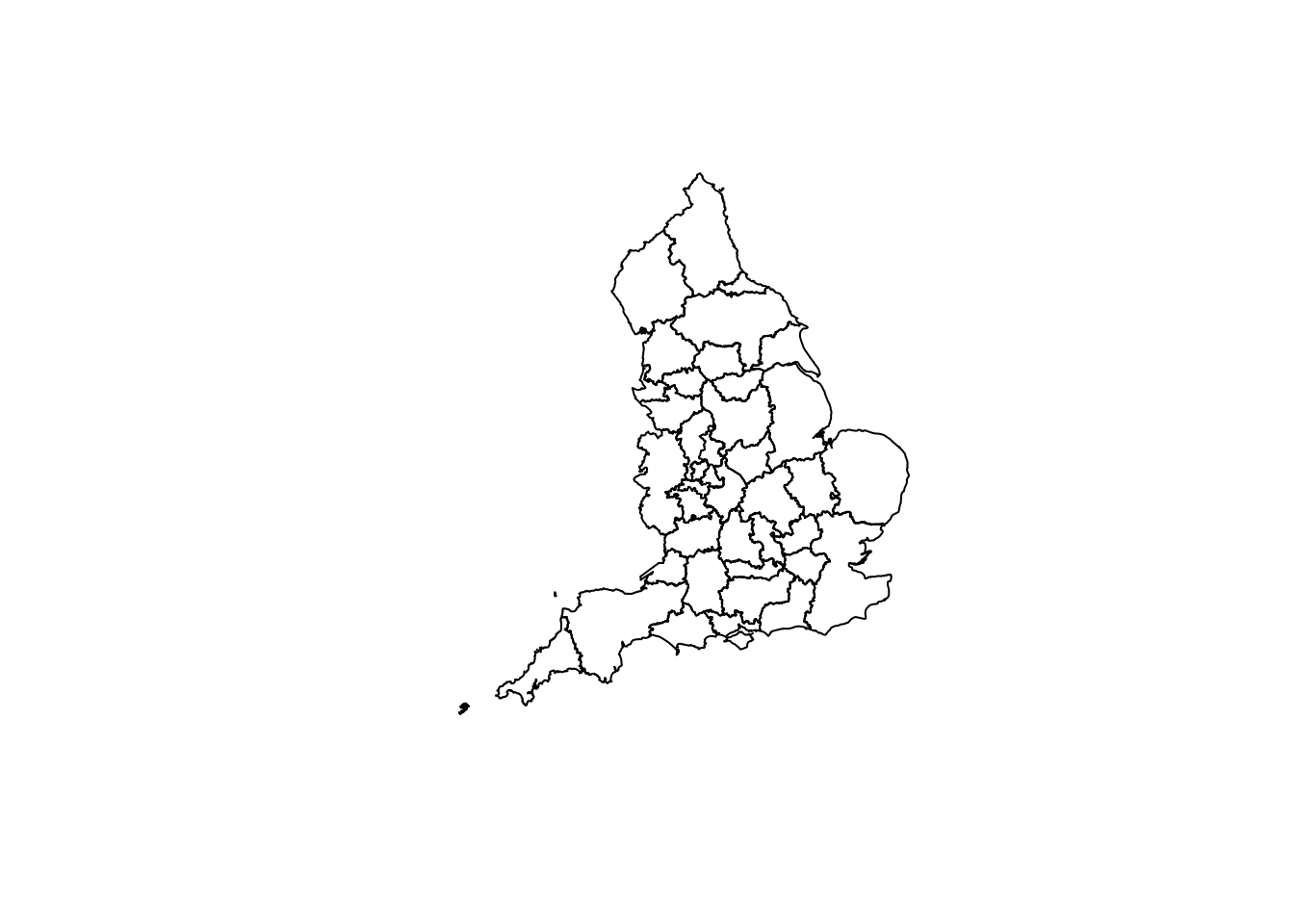

5.5 Bonus: Data Quality Assessment

Choose a dataset you have downloaded.
Assess its quality by checking for:
- Missing values
- Outliers
- Inconsistent data types
Document any issues found and how you would address them.

# Your code here

6 Further Reading

Reuse

CC BY-SA 4.0