STATS19

1 Introduction

This practical workbook guides you through the process of importing, processing and visualising STATS19 data using R with reference to a real-world case study: changes to the A58 in Leeds. Roundhay Road is a major road which runs from central Leeds to Rounday Park in the North of the city. The changes focus on the southern part of Roundhay Road around its intersections with Bayswater Road and Spencer Place, as highlighted in the consultation “Have Your Say Today - A58 Improvements - Commonplace” and illustrated in Figure 1.

Figure 1: Overview of changes to the southern section of Roundhay road proposed by Connecting Leeds in 2025. Credit: Leeds City Council.

2 Setup and prerequisites

We will use packages listed in the following code chunk to reproduce the analysis. Run the code chunk below to install and load the required packages.

options(repos = c(CRAN = "https://cloud.r-project.org"))
if (!require("remotes")) install.packages("remotes")
pkgs = c(
    "sf",
    "tidyverse",
    "tmap",
    "data.table",
    "stats19"
)

remotes::install_cran(pkgs)
sapply(pkgs, require, character.only = TRUE)
        sf  tidyverse       tmap data.table    stats19 
      TRUE       TRUE       TRUE       TRUE       TRUE 

See the prerequisites page for details and to test your setup.

3 Results presented in the consultation

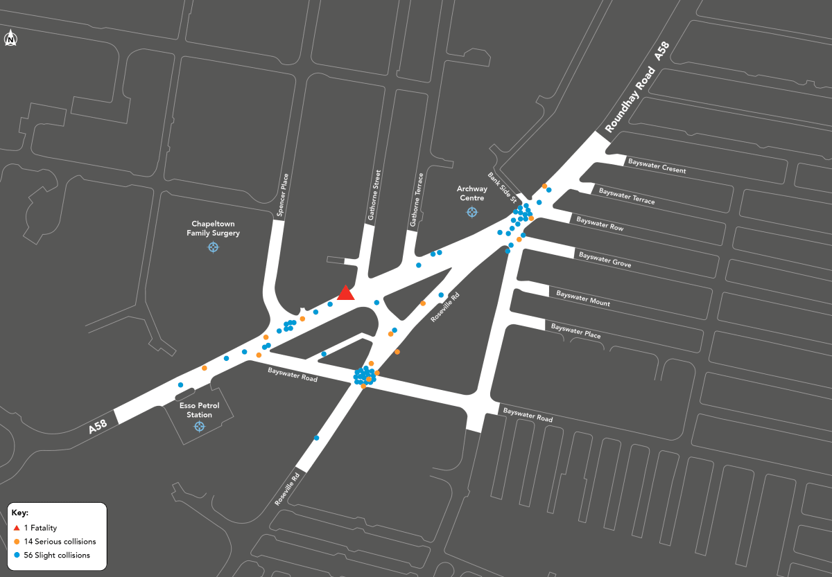
Step 4 of the consultation contains the map presented in Figure 2.

Figure 2: Map of collisions in the study area. Credit: Leeds City Council

Let’s try to reproduce the map.

4 Defining study area

There are different ways to define the study area. We could manually look it up but geocoding may be a better approach. Looking at the area on Google Maps shows that Cross Roseville Road is roughly in the centre of the study area:

study_coords = stplanr::geo_code("Cross Roseville Road, Leeds")

That gives us the coordinates we need, which could also be obtained using other geocoding services or added manually as follows:

study_coords = c(-1.5243862, 53.8109931)

Convert the coordinates to an sf object as follows, remembering to add the coordinate reference system (CRS):

study_point <- study_coords |>
  st_point() |>
  sf::st_sfc() |>
  sf::st_sf(geometry = _, crs = "EPSG:4326") 
study_point
Simple feature collection with 1 feature and 0 fields
Geometry type: POINT
Dimension:     XY
Bounding box:  xmin: -1.524386 ymin: 53.81099 xmax: -1.524386 ymax: 53.81099
Geodetic CRS:  WGS 84
                    geometry
1 POINT (-1.524386 53.81099)

Note: the |> symbol above is R’s ‘native pipe’ which passes the result of the left-hand side expression to the right-hand side expression as the first argument, allowing for more readable and concise code. The _ symbol refers to the current object being processed in the pipeline.

Let’s define a buffer around our point. There isn’t a scale bar in the original map, so it’s hard to know the exact distance to use for the buffer. However, we can start with a 500 meter buffer.

study_buffer <- study_point |>
  st_buffer(dist = 500)

tm_shape(study_buffer)+
  tm_fill("gray80",fill_alpha = 0.8)+
  tm_shape(study_point)+
  tm_dots()

collision_data <- lapply(2019:2024,
                         get_stats19,
                         type = "collision",
                         silent = TRUE,
                         output_format = "sf") |> 
  bind_rows()
date and time columns present, creating formatted datetime column
28 rows removed with no coordinates
date and time columns present, creating formatted datetime column
14 rows removed with no coordinates
date and time columns present, creating formatted datetime column
17 rows removed with no coordinates
date and time columns present, creating formatted datetime column
22 rows removed with no coordinates
date and time columns present, creating formatted datetime column
12 rows removed with no coordinates
date and time columns present, creating formatted datetime column
84 rows removed with no coordinates

An inspection of the data

names(collision_data)
 [1] "accident_index"                              
 [2] "accident_year"                               
 [3] "accident_reference"                          
 [4] "longitude"                                   
 [5] "latitude"                                    
 [6] "police_force"                                
 [7] "accident_severity"                           
 [8] "number_of_vehicles"                          
 [9] "number_of_casualties"                        
[10] "date"                                        
[11] "day_of_week"                                 
[12] "time"                                        
[13] "local_authority_district"                    
[14] "local_authority_ons_district"                
[15] "local_authority_highway"                     
[16] "first_road_class"                            
[17] "first_road_number"                           
[18] "road_type"                                   
[19] "speed_limit"                                 
[20] "junction_detail"                             
[21] "junction_control"                            
[22] "second_road_class"                           
[23] "second_road_number"                          
[24] "pedestrian_crossing_human_control"           
[25] "pedestrian_crossing_physical_facilities"     
[26] "light_conditions"                            
[27] "weather_conditions"                          
[28] "road_surface_conditions"                     
[29] "special_conditions_at_site"                  
[30] "carriageway_hazards"                         
[31] "urban_or_rural_area"                         
[32] "did_police_officer_attend_scene_of_accident" 
[33] "trunk_road_flag"                             
[34] "lsoa_of_accident_location"                   
[35] "enhanced_severity_collision"                 
[36] "datetime"                                    
[37] "geometry"                                    
[38] "status"                                      
[39] "collision_index"                             
[40] "collision_year"                              
[41] "collision_reference"                         
[42] "legacy_collision_severity"                   
[43] "did_police_officer_attend_scene_of_collision"
[44] "lsoa_of_collision_location"                  

Let’s reconcile some data to match the appropriate convention

collision_data <- collision_data |> 
  mutate(collision_year = coalesce(collision_year,accident_year),
         legacy_collision_severity = coalesce(legacy_collision_severity,accident_severity))

Let’s visualise all the data we extracted

collision_data |>
  slice_sample(n = 5000) |>
  st_geometry() |> 
  tm_shape()+
  tm_dots()

Creating a subset of the collisions within our study area

st_crs(collision_data,)
Coordinate Reference System:
  User input: EPSG:27700 
  wkt:
PROJCRS["OSGB36 / British National Grid",
    BASEGEOGCRS["OSGB36",
        DATUM["Ordnance Survey of Great Britain 1936",
            ELLIPSOID["Airy 1830",6377563.396,299.3249646,
                LENGTHUNIT["metre",1]]],
        PRIMEM["Greenwich",0,
            ANGLEUNIT["degree",0.0174532925199433]],
        ID["EPSG",4277]],
    CONVERSION["British National Grid",
        METHOD["Transverse Mercator",
            ID["EPSG",9807]],
        PARAMETER["Latitude of natural origin",49,
            ANGLEUNIT["degree",0.0174532925199433],
            ID["EPSG",8801]],
        PARAMETER["Longitude of natural origin",-2,
            ANGLEUNIT["degree",0.0174532925199433],
            ID["EPSG",8802]],
        PARAMETER["Scale factor at natural origin",0.9996012717,
            SCALEUNIT["unity",1],
            ID["EPSG",8805]],
        PARAMETER["False easting",400000,
            LENGTHUNIT["metre",1],
            ID["EPSG",8806]],
        PARAMETER["False northing",-100000,
            LENGTHUNIT["metre",1],
            ID["EPSG",8807]]],
    CS[Cartesian,2],
        AXIS["(E)",east,
            ORDER[1],
            LENGTHUNIT["metre",1]],
        AXIS["(N)",north,
            ORDER[2],
            LENGTHUNIT["metre",1]],
    USAGE[
        SCOPE["Engineering survey, topographic mapping."],
        AREA["United Kingdom (UK) - offshore to boundary of UKCS within 49°45'N to 61°N and 9°W to 2°E; onshore Great Britain (England, Wales and Scotland). Isle of Man onshore."],
        BBOX[49.75,-9.01,61.01,2.01]],
    ID["EPSG",27700]]
st_crs(study_buffer)
Coordinate Reference System:
  User input: EPSG:4326 
  wkt:
GEOGCRS["WGS 84",
    ENSEMBLE["World Geodetic System 1984 ensemble",
        MEMBER["World Geodetic System 1984 (Transit)"],
        MEMBER["World Geodetic System 1984 (G730)"],
        MEMBER["World Geodetic System 1984 (G873)"],
        MEMBER["World Geodetic System 1984 (G1150)"],
        MEMBER["World Geodetic System 1984 (G1674)"],
        MEMBER["World Geodetic System 1984 (G1762)"],
        MEMBER["World Geodetic System 1984 (G2139)"],
        ELLIPSOID["WGS 84",6378137,298.257223563,
            LENGTHUNIT["metre",1]],
        ENSEMBLEACCURACY[2.0]],
    PRIMEM["Greenwich",0,
        ANGLEUNIT["degree",0.0174532925199433]],
    CS[ellipsoidal,2],
        AXIS["geodetic latitude (Lat)",north,
            ORDER[1],
            ANGLEUNIT["degree",0.0174532925199433]],
        AXIS["geodetic longitude (Lon)",east,
            ORDER[2],
            ANGLEUNIT["degree",0.0174532925199433]],
    USAGE[
        SCOPE["Horizontal component of 3D system."],
        AREA["World."],
        BBOX[-90,-180,90,180]],
    ID["EPSG",4326]]

Let’s transform the buffer to match the British Grid

study_buffer_BNG <- study_buffer |> st_transform(st_crs(collision_data))
study_collisions <- collision_data[study_buffer_BNG,]

A quick exploration of the amount

study_collisions |>
  count(legacy_collision_severity)
Simple feature collection with 2 features and 2 fields
Geometry type: MULTIPOINT
Dimension:     XY
Bounding box:  xmin: 430986 ymin: 434604 xmax: 431916 ymax: 435550
Projected CRS: OSGB36 / British National Grid
# A tibble: 2 × 3
  legacy_collision_severity     n                                       geometry
* <chr>                     <int>                               <MULTIPOINT [m]>
1 Serious                      32 ((431178 435174), (431239 434801), (431262 43…
2 Slight                      109 ((430986 434873), (431028 434897), (431110 43…

A quick visualisation

study_collisions |>
tm_shape()+
  tm_dots(fill = "legacy_collision_severity",
          size = 1,
          fill_alpha = 0.7,
          fill.scale = tm_scale_categorical(
            labels = c("Slight","Serious"),
            values = c("orange","dodgerblue")))

A better version

study_collisions |>
  mutate(legacy_collision_severity = factor(legacy_collision_severity,
                                            c("Slight","Serious","Fatal"),
                                            ordered = T)) |>
  arrange(legacy_collision_severity) |> 
  mutate(X = st_coordinates(geometry)[,1],
         Y = st_coordinates(geometry)[,2]) |> 
  ggplot(aes(x = X,y = Y,col = legacy_collision_severity))+
  geom_jitter(alpha = 0.8,
              size = 2,
              position = position_jitter(width = 5, height = 5))+
  theme_void()+
  scale_color_manual(values = c("dodgerblue","orange","red"))+
  theme(plot.background = element_rect(fill = "gray20"))

Reuse